PSTAT 5A: Lecture 18

Correlation, and an Intro to Regression

Ethan P. Marzban

2023-06-01

Review of Relevant Lecture 02 Material

Scatterplots and Trends

• Recall, from Lecture 2, that the best type of plot to visualize the relationship between to numerical variables is a scatterplot.

• Based on the scatterplot, we can determine whether or not the two variables have an association (a.k.a. trend) or not.

• Associations can be positive or negative, and linear or nonlinear (or, not present at all)

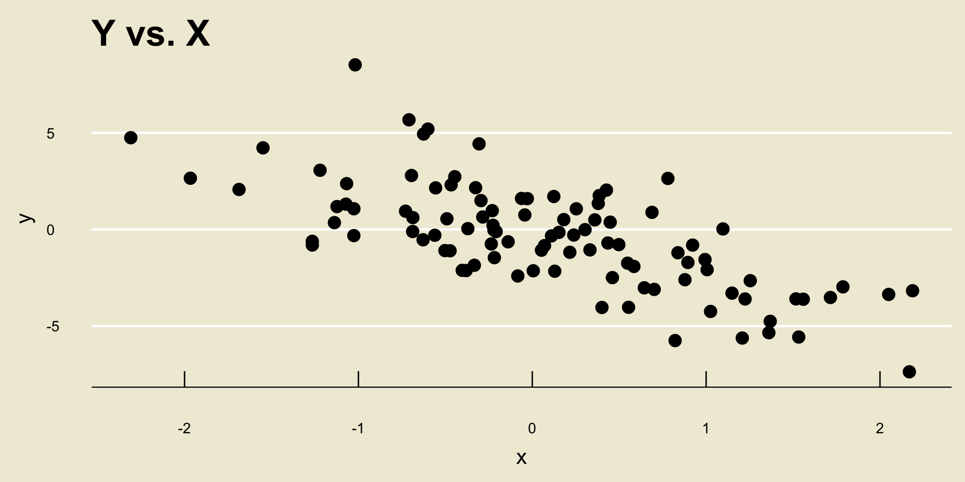
• Linear Negative Association:

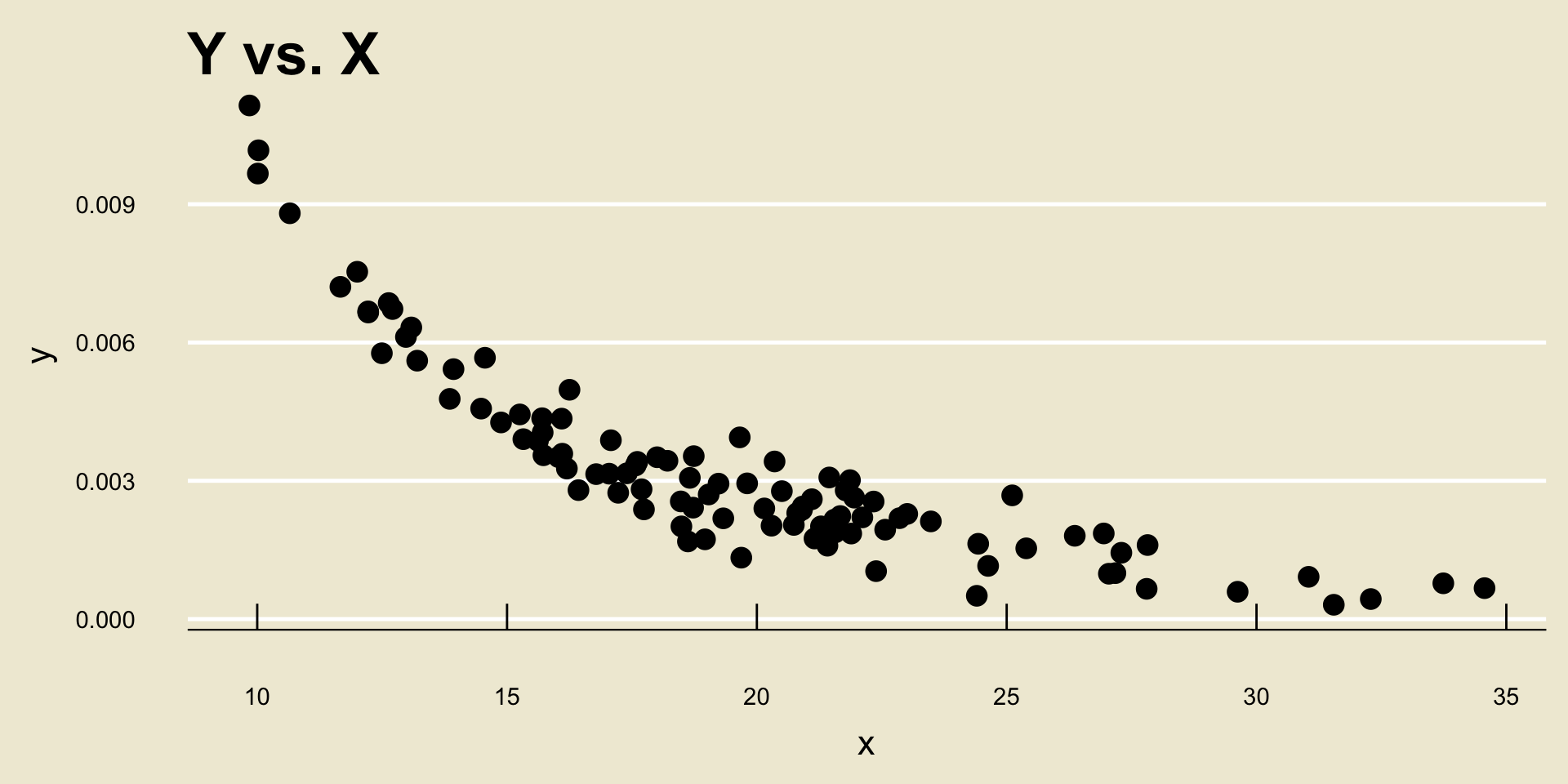
• Nonlinear Negative Association:

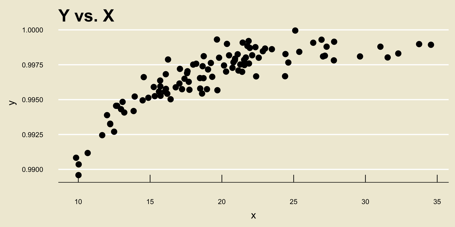
• Linear Positive Association:

• Nonlinear Positive Association:

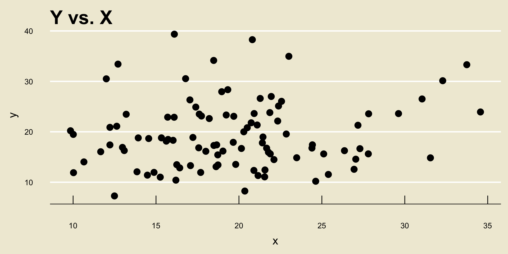
No Relationship

• Sometimes, two variables will have no relationship at all:

Strength of a Relationship

• There is another thing to be aware of.

• For example, consider the following two scatterplots:

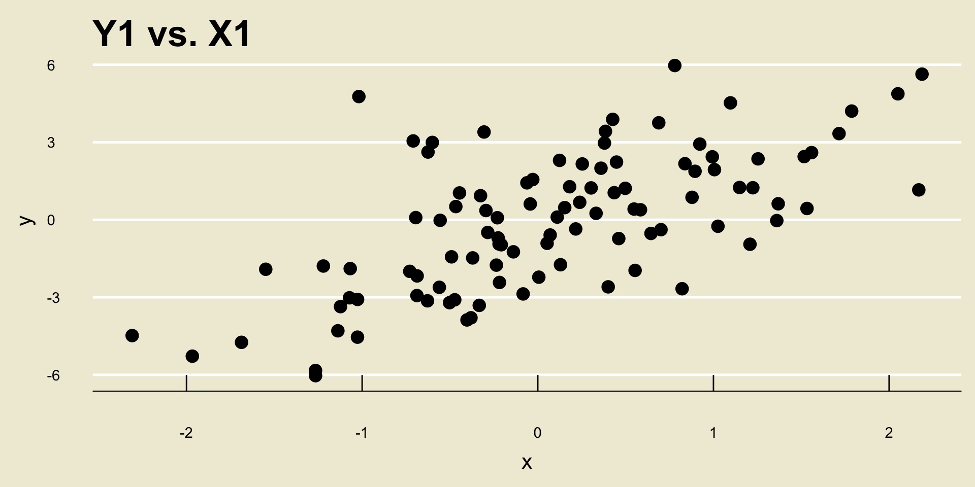
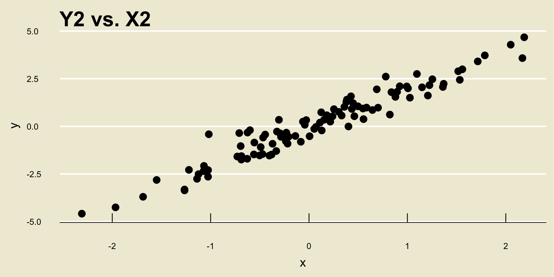
• Both scatterplots display a positive linear trend. However, the relationship between Y2 and X2 seems to be “stronger” than the relationship between Y1 and X1, does it not?

Correlation Coefficient

• Ultimately, we would like to develop a mathematical metric to quantify not only the relationship between two variables, but also the strength of the relationship between these two variables.

• This quantity is referred to as the correlation coefficient.

• Now, it turns out there are actually a few different correlation coefficients out there. The one we will use in this class (and one of the metrics that is very widely used by statisticians) is called Pearson’s Correlation Coefficient, or often just Pearson’s r (as we use the letter r to denote it.)

Pearson’s r

• Given two sets \(X = \{y_i\}_{i=1}^{n}\) and \(Y = \{y_i\}_{i=1}^{n}\) (note that we require the two sets to have the same number of elements!), we compute r using the formula \[ r = \frac{1}{n - 1} \sum_{i=1}^{n} \left( \frac{x_i - \overline{x}}{s_X} \right) \left( \frac{y_i - \overline{y}}{s_Y} \right) \] where:

  • \(\overline{x}\) and \(\overline{y}\) denote the sample means of \(X\) and \(Y\), respectively
  • \(s_X\) and \(s_Y\) denote the sample standard deviations of \(X\) and \(Y\), respectively.

Example

• I find it useful to sometimes consider extreme cases, and ensure that the math matches up with our intuition.

• For example, consider the sets \(X = \{1, 2, 3\}\) and \(Y = \{1, 2, 3\}\).

• From a scatterplot, I think we would all agree that \(X\) and \(Y\) have a positive linear relationship, and that the relationship is very strong!

Example

• Indeed, \(\overline{x} = 2 = \overline{y}\) and \(s_X = 1 = s_Y\), meaning \[\begin{align*} r & = \frac{1}{3 - 1} \left[ \left( \frac{1 - 2}{1} \right) \left( \frac{1 - 2}{1} \right) + \left( \frac{2 - 2}{1} \right) \left( \frac{2 - 2}{1} \right) \right. \\ & \hspace{45mm} \left. + \left( \frac{3 - 2}{1} \right) \left( \frac{3 - 2}{1} \right) \right] \\ & = \frac{1}{2} \left[ 1 + 0 + 1 \right] = \boxed{1} \end{align*}\]

• It turns out, r will always be between \(-1\) and \(1\), inclusive, regardless of what two sets we are comparing!

Interpretation

• So, here is how we interpret the value of r.

  • The sign of r (i.e. whether it is positive or negative) indicates whether or not the linear association between the two variables is positive or negative.

  • The magnitude of r indicates how strong the linear relationship between the two variables is, with magnitudes close to \(1\) or \(-1\) indicating very strong linear relationships.

  • An r value of 0 indicates no linear relationship between the variables.

Important Distinction

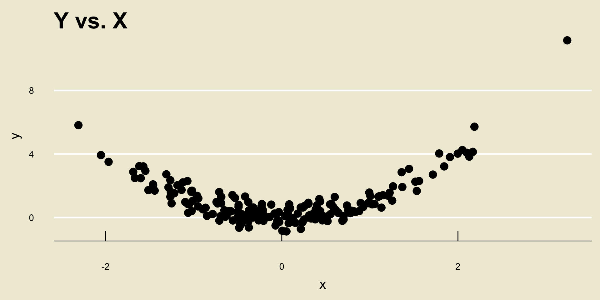
• Now, something that is very important to mention is that r only quantifies linear relationships- it is very bad at quantifying nonlinear relationships.

• For example, consider the following scatterplot:

Important Distinction

• I think we would all agree that Y and X have a fairly strong relationship.

• However, the correlation between Y and X is actually only 0.1953333!

• So, again- r should only be used as a determination of the strength of linear trends, not nonlinear trends.

Your Turn!

Your Turn!

Exercise 1

Compute the correlation between the following two sets of numbers: \[\begin{align*} \boldsymbol{x} & = \{-1, \ 0, \ 1\} \\ \boldsymbol{y} & = \{1, \ 2, \ 0\} \end{align*}\]

Leadup

• There is another thing to note about correlation.

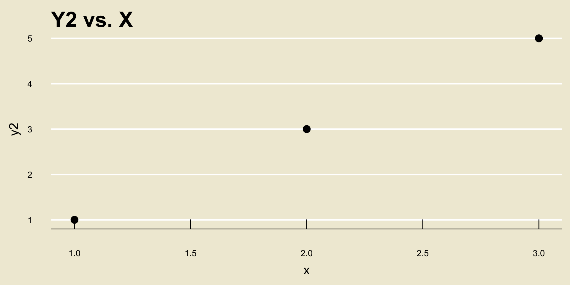
• Let’s see this by way of an example: consider the following two scatterplots:

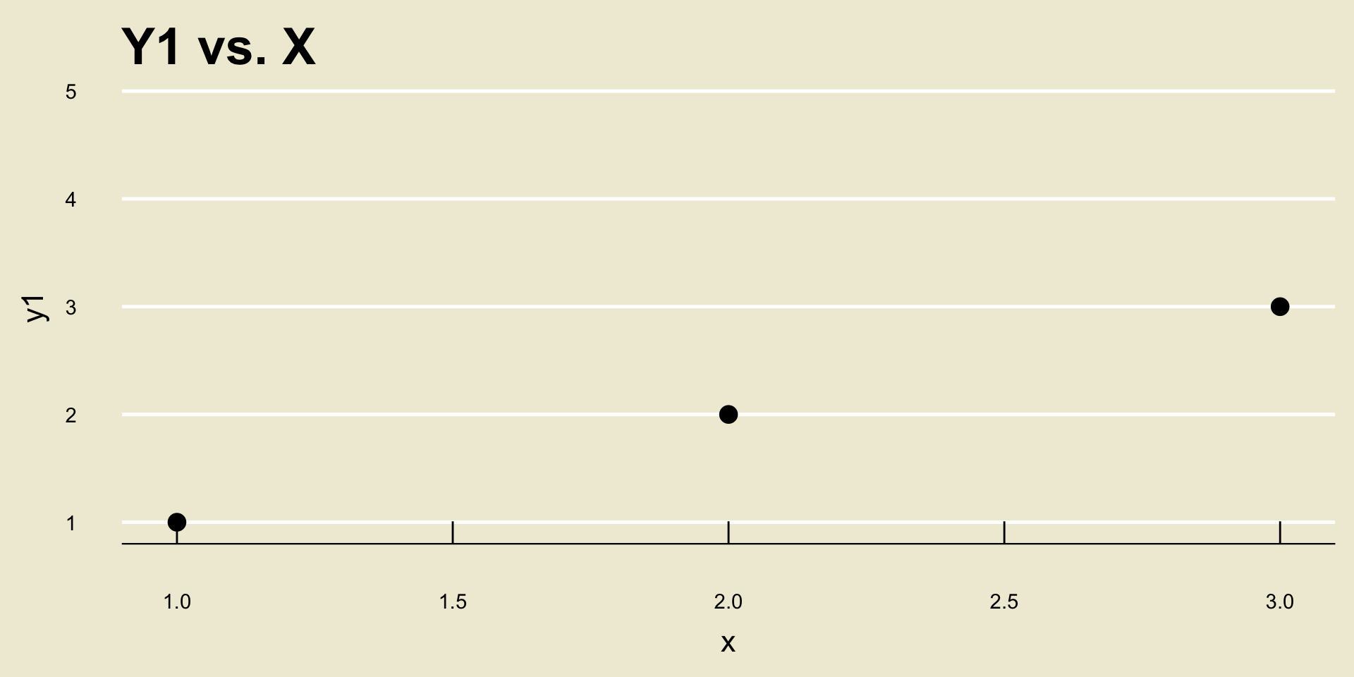
• Both cor(X, Y1) and cor(X, Y2) are equal to 1, despite the fact that a one unit increase in x corresponds to a different unit increase in y1 as opposed to y2.

Leadup

• So, don’t be fooled- the magnitude of r says nothing about how a one-unit increase in x translates to a change in y!

  • Again, the magnitude of r only tells us how strongly the two variables are related.

• A natural question that arises is then: how can we specify how a change in x translates to a change in y?

Leadup

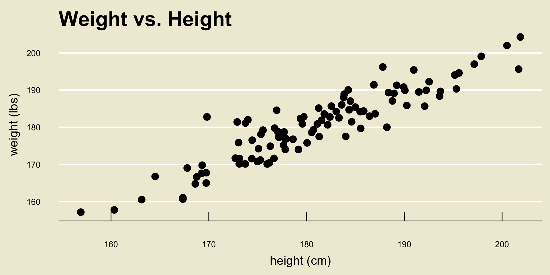
• To help ground our discussion, let’s think in terms of height and weight. That is, let x denote height and y denote weight.

• We would certainly expect some sort of positive association between height and weight (taller people tend to weigh slightly more than shorter people).

• But, if we were to take a series of observations on height and weight, and plot these observations on a scatterplot, we would not get data that is perfectly linear.

• Rather, we can imagine that there does exist some true linear “fit” (or “trend”) between height and weight, but randomness would inject some “error” into our data causing our data to be modeled as something like \[ \texttt{weight} = f(\texttt{height}) + \texttt{noise} \] where, in this case, we would expect the function \(f()\) to be a linear function.

Leadup

Leadup

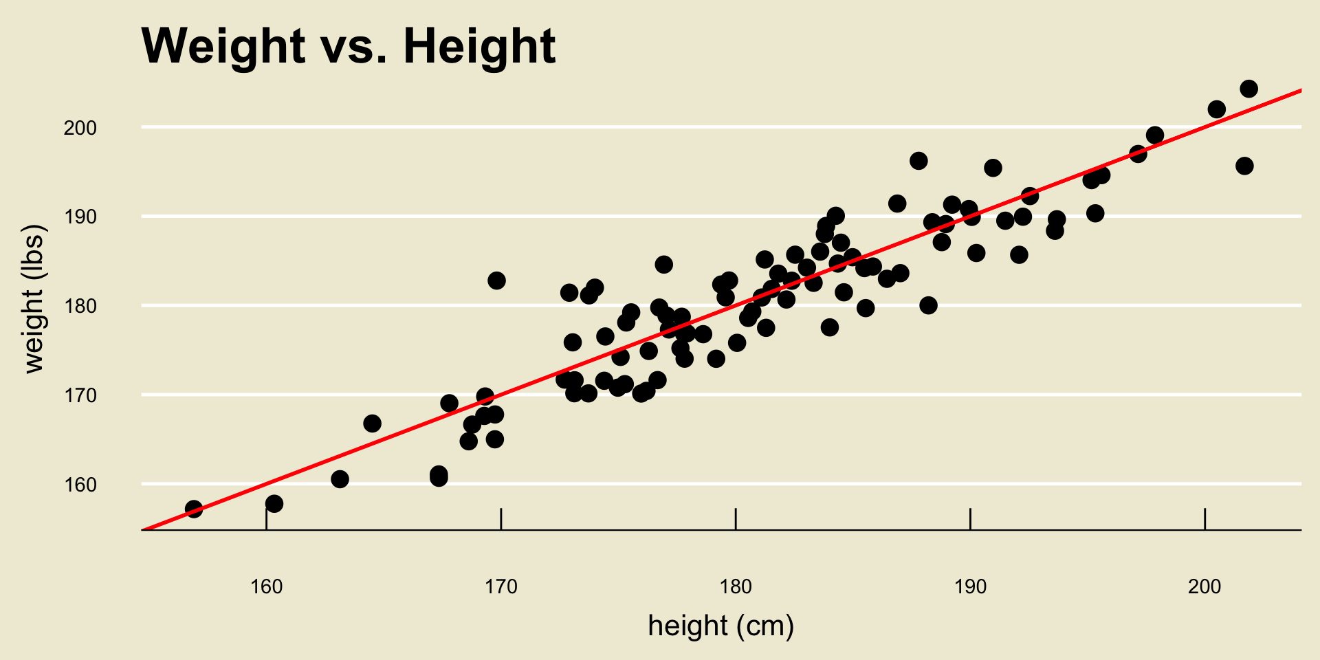
• Here, the red line represents the true relationship between height and weight, and any deviations from the line are assumed to be due to chance.

Leadup

• Recall that a line is specified by an intercept and a slope. Therefore, since we are assuming a linear relationship between height and weight, our model can be expressed as \[ \texttt{weight} = \beta_0 + \beta_1 \cdot \texttt{height} + \texttt{noise} \]

• In this way, we can see that \(\beta_0\) and \(\beta_1\) are effectively population parameters.

• Our next goal will be to find suitable estimators, \(\widehat{\beta_0}\) and \(\widehat{\beta_1}\), of \(\beta_0\) and \(\beta_1\), respectively.

Simple Linear Regression

Model

• In general, the goal of regression is to quantify the relationship between two variables, x and y.

• We call y the response variable and x the explanatory variable.

  • So, for example, in our height and weight example from above, weight was the response variable and height was the explanatory variable.

• Our model (assuming a linear relationship between x and y), is then \[ \texttt{y} = \beta_0 + \beta_1 \cdot \texttt{x} + \texttt{Noise} \]

Goals

• Here’s a visual way of thinking about what I said on the previous slide. Consider the following scatterplot:

Goals

• We are assuming that there exists some true linear relationship (i.e. some “fit”) between Y and X. But, because of natural variability due to randomness, we cannot figure out exactly what the true relationship is.

Goals

• Finding the “best” estimate of the fit is, therefore, akin to finding the line that “best” fits the data.

Line of Best Fit

• Now, if we are to find the line that best fits the data, we first need to quantify what we mean by “best”.

• Here is one idea: consider minimizing the average distance from the datapoints to the line.

• As a measure of “average distance from the points to the line”, we will use the so-called residual sum of squares (often abbreviated as RSS).

Residuals

• The i^th residual is defined to be the quantity \(e_i\) below:

• RSS is then just \(\displaystyle \mathrm{RSS} = \sum_{i=1}^{n} e_i^2\)

Results

• It turns out, using a bit of Calculus, the estimators we seek (i.e. the ones that minimize the RSS) are \[\begin{align*} \widehat{\beta_1} & = \frac{\sum\limits_{i=1}^{n} (x_i - \overline{x})(y_i - \overline{y})}{\sum\limits_{i=1}^{n} (x_i - \overline{x})^2} \\ \widehat{\beta_0} & = \overline{y} - \widehat{\beta_1} \overline{x} \end{align*}\]

• These are what are known as the ordinary least squares estimators of \(\beta_0\) and \(\beta_1\), and the line \(\widehat{\beta_0} + \widehat{\beta_1} x\) is called the least-squares regression line.

• Perhaps an example may illustrate what I am talking about.

Example

Example

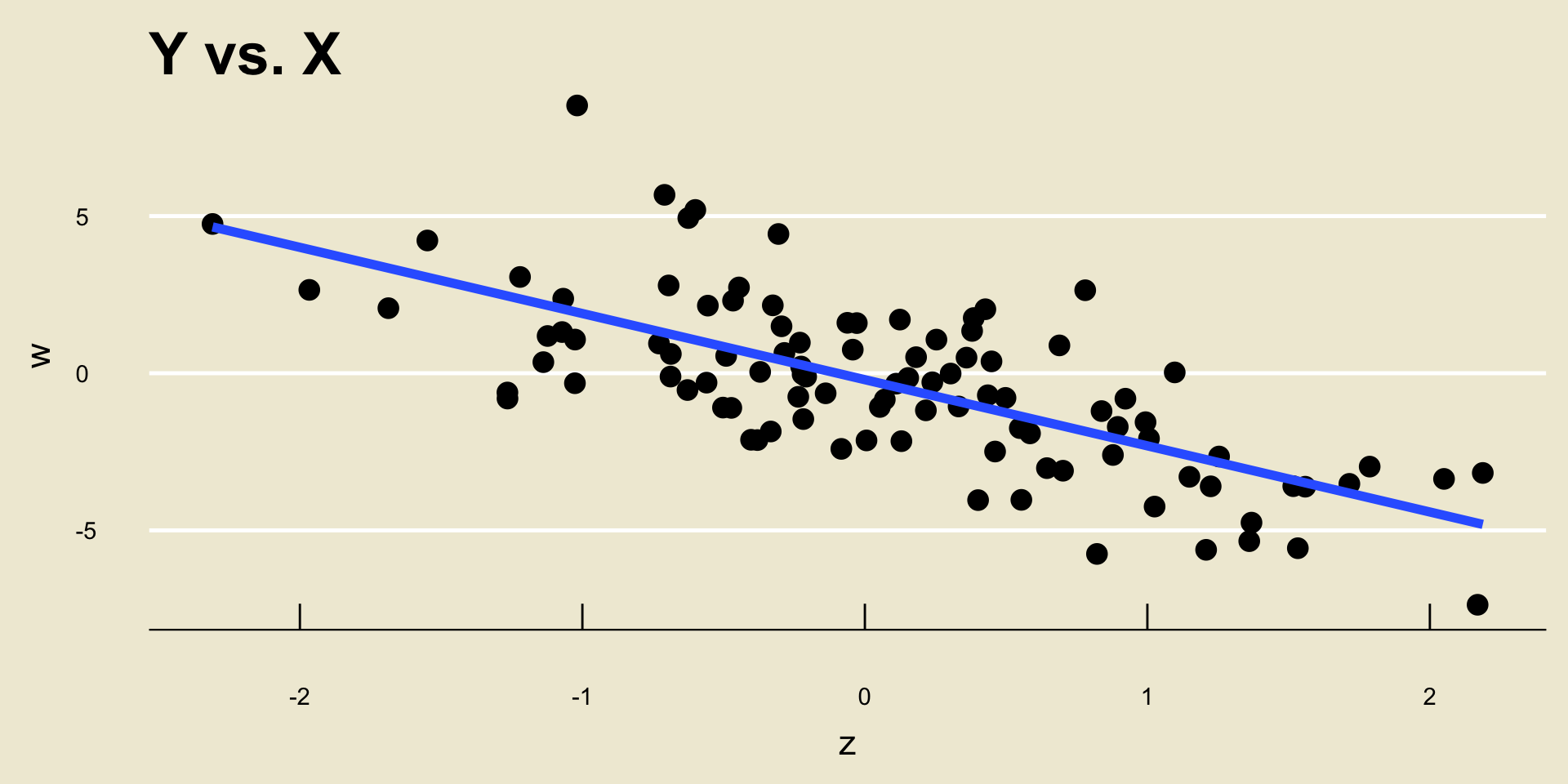
• \(\widehat{\beta_0} =\) -0.2056061; \(\widehat{\beta_1} =\) -2.1049432.

• I.e. the equation of the line in blue is -0.2056061 + -2.1049432 * x.

Fitted Values

• Let’s return to our cartoon picture of OLS regression:

Fitted Values

• Notice that each point in our dataset (i.e. the blue points) have a corresponding point on the OLS regression line:

Fitted Values

• These points are referred to as fitted values; the y-values of the fitted values are denoted as \(\widehat{y}_i\).

• In this way, the OLS regression line is commonly written as a relationship between the fitted values and the x-values: \[ \widehat{y} = \widehat{\beta_0} + \widehat{\beta_1} x \]

Back to height and weight

• Before we work through the math once, let’s apply this technique to the height and weight data from before.

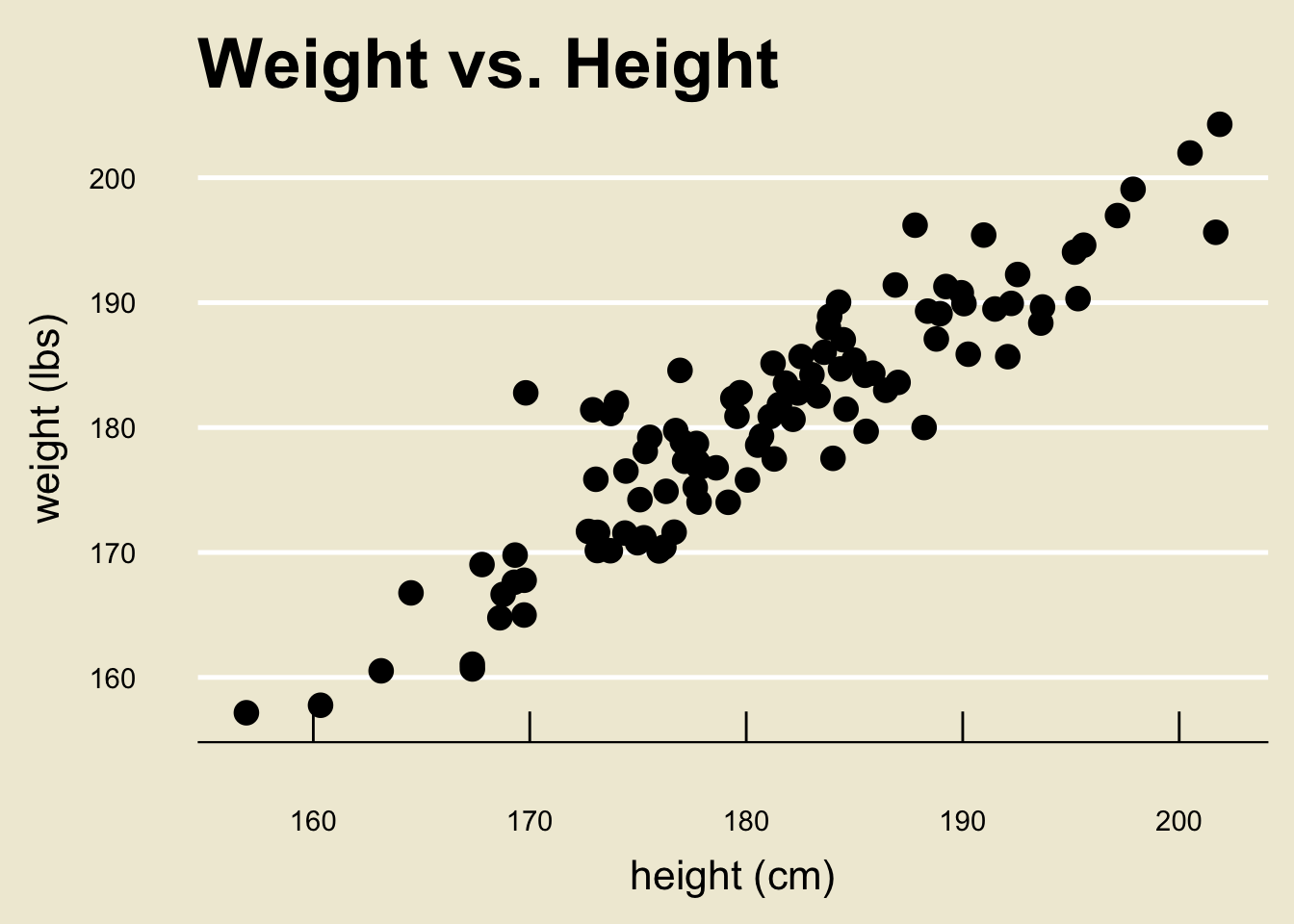
Back to height and weight

• Using a computer software, the OLS regression line can be found to be:

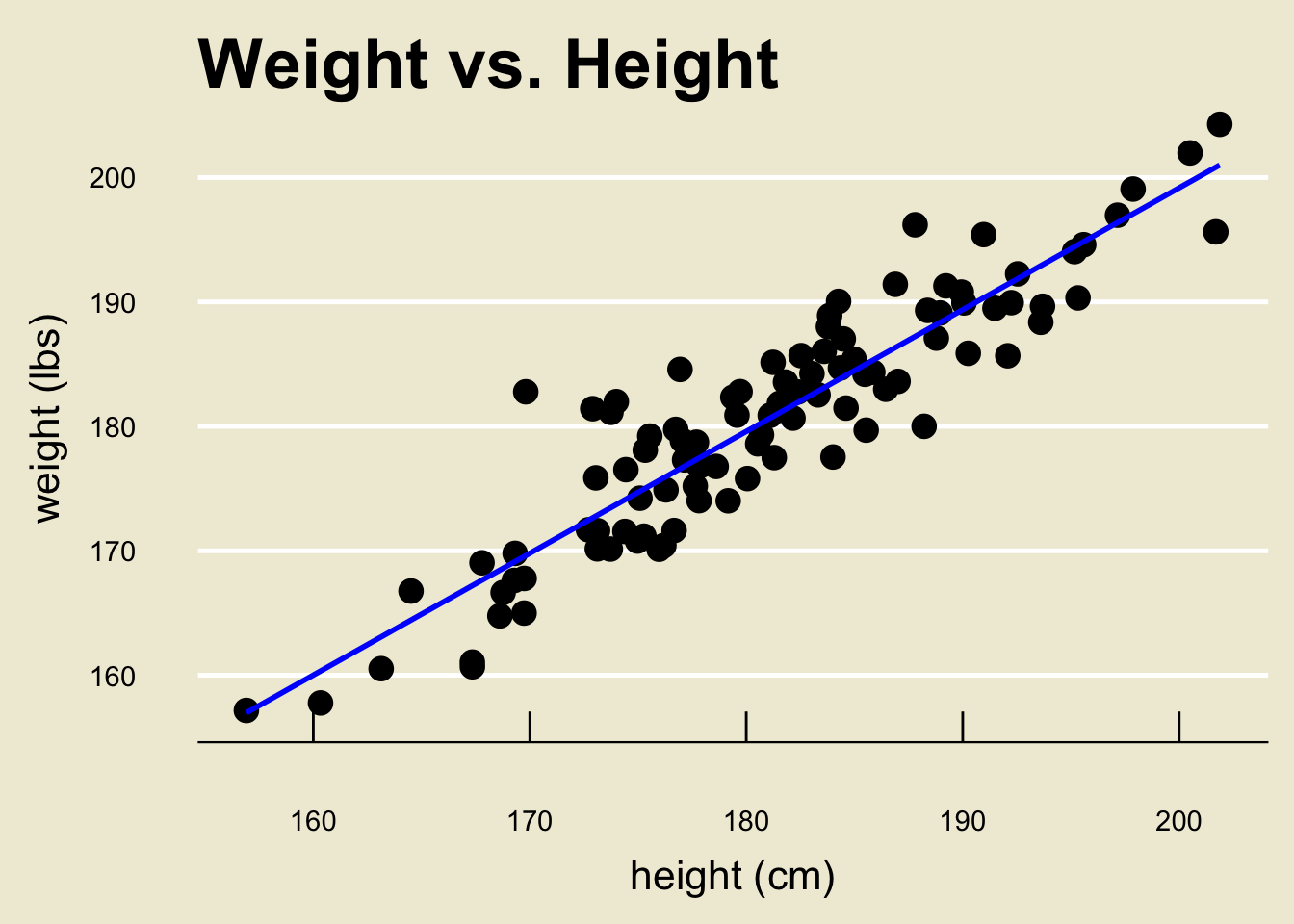
• Specifically, \(\widehat{\beta_0} =\) 3.366744 and \(\widehat{\beta_1} =\) 0.9790114

• We will return to the notion of fitted values in a bit.

Back to height and weight

• A quick note:

• Though there was no way to know this, the true \(\beta_1\) was actually \(1.0\). Again, this is just to demonstrate that the OLS estimate \(\widehat{\beta_1}\) is just that- an estimate!

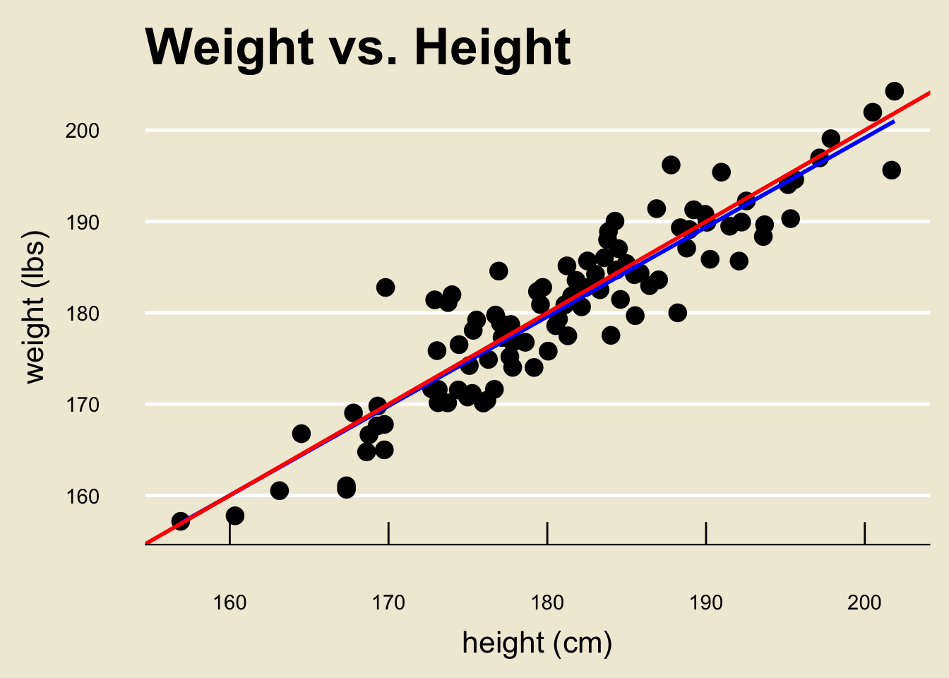
\[ \widehat{\texttt{weight}} = 3.367 + 0.979 \cdot \texttt{height} \]

Worked-Out Example

• Alright, let’s work through a computation by hand once.

• Suppose we have the variables \[\begin{align*} \boldsymbol{x} & = \{3, \ 7, \ 8\} \\ \boldsymbol{y} & = \{20, \ 14, \ 17\} \end{align*}\] and suppose we wish to construct the least-squares regression line when regressing \(\boldsymbol{y}\) onto \(\boldsymbol{x}\).

• First, we compute \[\begin{align*} \overline{x} & = 6 \\ \overline{y} & = 17 \end{align*}\]

Worked-Out Example

• Next, we compute \[\begin{align*} \sum_{i=1}^{n} (x_i - \overline{x})^2 & = (3 - 6)^2 + (7 - 6)^2 + (8 - 6)^2 = 14 \\ \sum_{i=1}^{n} (y_i - \overline{y})^2 & = (20 - 17)^2 + (14 - 17)^2 + (17 - 17)^2 = 18 \end{align*}\]

• Additionally, \[\begin{align*} \sum_{i=1}^{n} (x_i - \overline{x})(y_i - \overline{y}) & = (3 - 6)(20 - 17) + (7 - 6)(14 - 17) \\[-7mm] & \hspace{10mm} + (8 - 6)(17 - 17) \\[5mm] & = -12 \end{align*}\]

Worked-Out Example

• Therefore, \[ \widehat{\beta_1} = \frac{\sum_{i=1}^{n} (x_i - \overline{x})(y_i - \overline{y})}{\sum_{i=1}^{n} (x_i - \overline{x})^2} = \frac{-12}{14} = - \frac{6}{7} \]

• Additionally, \[ \widehat{\beta_0} = \overline{y} - \widehat{\beta_1} \overline{x} = 17 - \left( - \frac{6}{7} \right) (6) = \frac{155}{7} \]

• This means that the ordinary least-squares regression line is \[ \boxed{\widehat{y} = \frac{1}{7} ( 155 - 6 x )} \]

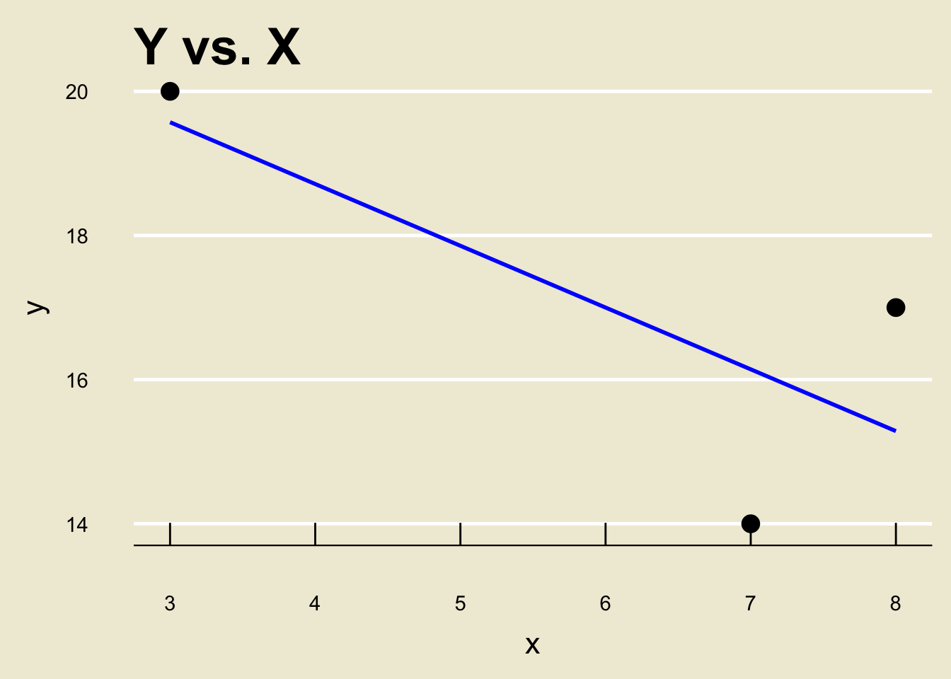
\[ \widehat{y} = \frac{1}{7} ( 155 - 6 x ) \]

Interpreting the Coefficients

• Alright, so how do we interpret the OLS regression line? \[\widehat{y} = \widehat{\beta_0} + \widehat{\beta_1} x\]

• We can see that a one-unit increase in x corresponds to a \(\widehat{\beta_1}\)-unit increase in y.

  • For example, in our height and weight example we found \[ \widehat{\texttt{weight}} = 3.367 + 0.979 \cdot \texttt{height} \]

  • This means that a one-cm change in height is associated with a (predicted/estimated) 0.979 lbs change in weight.

Prediction

• We can also use the OLS regression line to perform prediction.

• To see how this works, let’s return to our toy example:

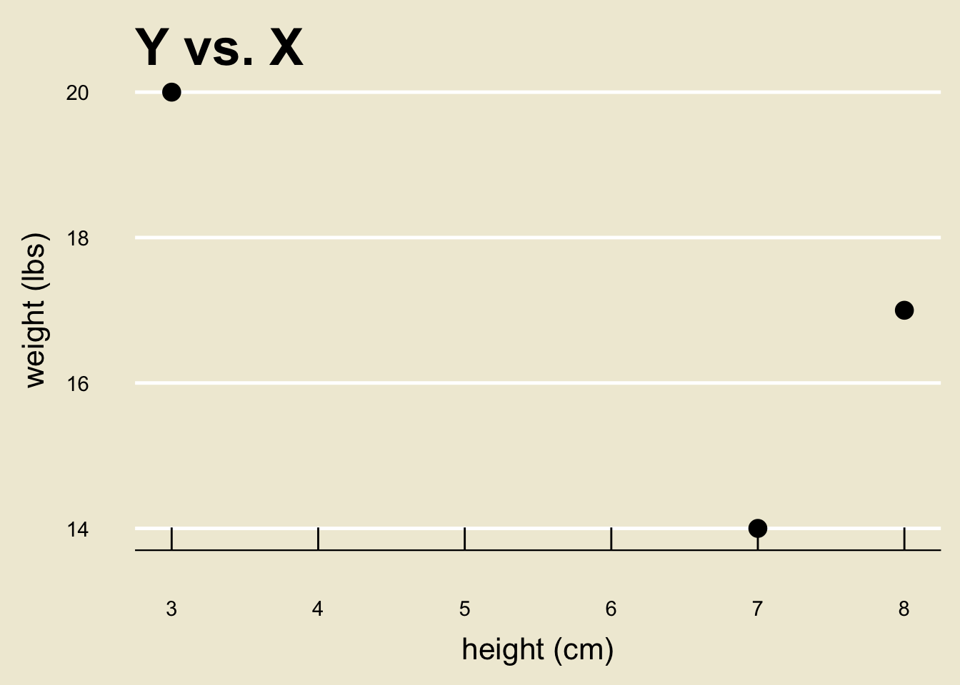
• Notice that we do not have an x-observation of 5. As such, we don’t know what the y-value corresponding to an x-value of 5 is.

Prediction

• However, we do have a decent guess as to what the y-value corresponding to an x-value of 5 is- the corresponding fitted value!

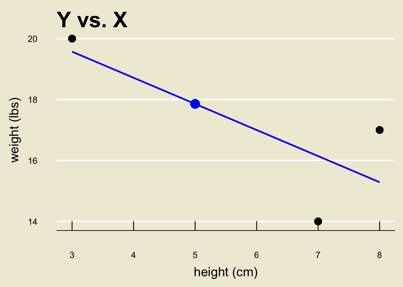
\[ \widehat{y}_5 = \frac{1}{7} (155 - 6 \cdot 5) \approx 17.857 \]

Extrapolation, and the Dangers Thereof

• Let’s look at another toy dataset:

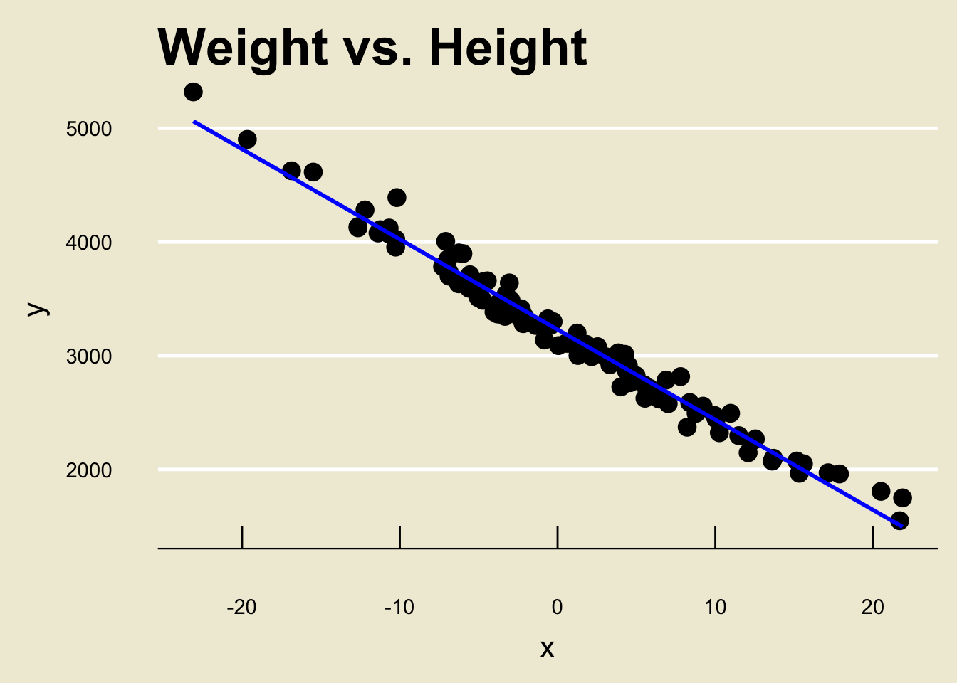
• Looks pretty linear, right?

Extrapolation, and the Dangers Thereof

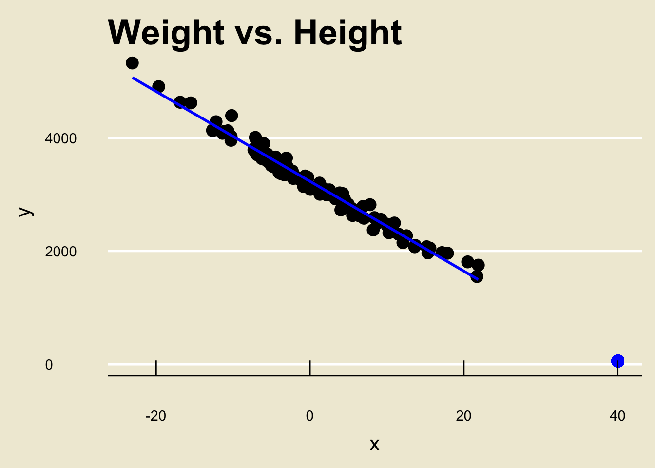
• Say we want to predict the corresponding y value of an x value of, 40.

• Following our steps from before, we would just find the fitted value corresponding to x = 40:

Extrapolation, and the Dangers Thereof

• Here’s the kicker: the true fit was actually NOT linear!

  • Specifically, I used a quadratic relationship between x and y to generate the data.

  • When you zoom in close enough, parabolas look linear!

• Now, we wouldn’t have had any way of knowing this.

• This is why it is a bad idea to try to extrapolate too far.

  • Extrapolation is the name we give to trying to apply a model estimate to values that are very far outside the realm of the original data.

  • How far is “very far”? Statisticians disagree on this front. For the purposes of this class, just use your best judgment.

One Final Connection

• Now, one final thing I’d like to mention: note that the slope of the OLS regression line is not just the correlation coefficient.

  • Again, the magnitude of the correlation coefficient just gives us a measure of how strong the relationship between the two variables is.

• There is, however, a relationship between \(\widehat{\beta_1}\) and r: it turns out that \[ \widehat{\beta_1} = \frac{s_Y}{s_X} \cdot r \]

• A question may arise: do we really believe our OLS estimate of the slope?

• Remember that \(\widehat{\beta_1}\) is just an estimator of \(\beta_1\).

  • Next time, we’ll talk about how to construct confidence intervals for \(\widehat{\beta_1}\).

Your Turn!

Exercise 2

An airline is interested in determining the relationship between flight duration (in minutes) and the net amount of soda consumed (in oz.). Letting x denote flight duration (the explanatory variable) and y denote amount of soda consumed (the response variable), a sample of size 100 yielded the following results: \[ \begin{array}{cc} \displaystyle \sum_{i=1}^{n} x_i = 10,\!211.7; & \displaystyle \sum_{i=1}^{n} (x_i - \overline{x})^2 = 38,\!760.68 \\ \displaystyle \sum_{i=1}^{n} y_i = 14,\!3995.8; & \displaystyle \sum_{i=1}^{n} (y_i - \overline{y})^2 = 87.23984 \\ \displaystyle \sum_{i=1}^{n} (x_i - \overline{x})(y_i - \overline{y}) = 379.945 \\ \end{array} \]

1. Find the equation of the OLS Regression line.
2. If a particular flight has a duration of 110 minutes, how many ounces of soda would we expect to be consumed on the flight?