PSTAT 5A: Lecture 10

Continuous Random Variables

Ethan P. Marzban

2023-07-11

Last Time

Last lecture we started talking about random variables.
A random variable is a numeric outcome of some random process or experiment.
- For example, “number of heads observed in \(5\) independent tosses of a fair coin”
The state space of a random variable \(X\) is the set \(S_X\) of possible values the random variable could attain.
- If \(S_X\) has jumps, we say \(X\) is a “discrete random variable”
- Otherwise, we say \(X\) is a “continuous random variable.”
Today we’ll talk about continuous random variables.

Rule-of-Thumb

Here is a quick way to determine whether a random variable is continuous or discrete:

If the random variable is something you can count, then it is discrete.
If the random variable is something you can measure, then it is continuous.

I’d like to stress, though- this is only a rule-of-thumb. If we ask you to justify your choice of classification of a random variable as either discrete or continuous, your argument must make mention of the state space (as this is the true definitional way of classifying random variables.)

Your Turn!

Exercise 1

Classify the following random variables as either discrete or continuous. Make sure to provide appropriate justification!

\(X =\) the number of times a computer program crashes in a given day.
\(Y =\) the height of a randomly-selected skyscraper in downtown Los Angeles
\(Z =\) the weight of a randomly-selected fish from a lake
\(W =\) the number of cats that are adopted out of the Santa Barbara location of the Santa Barbara Humane Society each year.

Continuous Random Variables

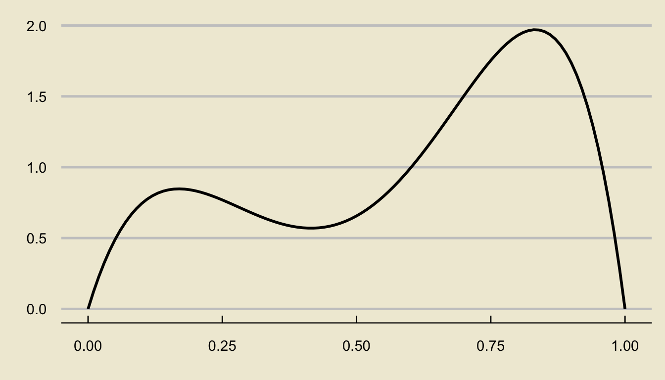
Continuous random variables are described by their so-called probability density function (or p.d.f. for short).
- The graph of a p.d.f. is called the density curve.
The p.d.f. is such that probabilities are found as areas underneath the density curve.
For example, if the random variable \(X\) has the following density curve…

…then the probability \(\mathbb{P}(0.25 \leq X \leq 0.75)\) is represented by the following area:

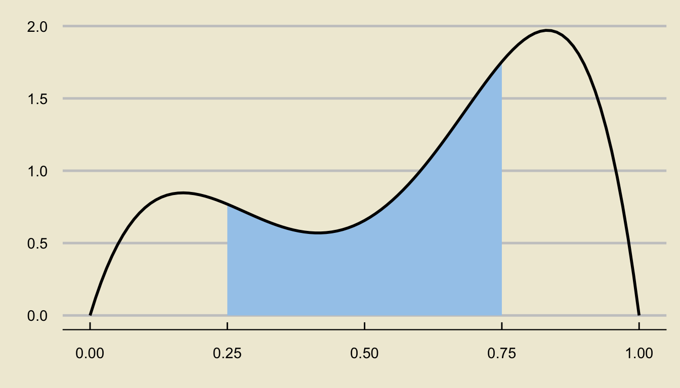
By the way, the state space of a continuous random variable can always be recovered from a density curve by finding the set of values over which the density curve is nonzero.

Two Properties

Since probabilities are areas underneath the density curve, we arrive at the following two properties (which themselves follow from the Axioms of Probability):

Properties of a P.D.F.

Density curves must always be nonnegative; i.e. the corresponding p.d.f. \(f_X(x)\) must obey \(f_X(x) \geq 0\) for every \(x\).
The area underneath a density curve must be \(1\).

In this lecture, we will examine two continuous distributions: the uniform distribution, and the normal distribution.
- We will see that the density curves/p.d.f.’s of these two distributions will satisfy the above two properties.

Uniform Distribution

The uniform distribution takes two parameters: \(a\) and \(b\), with \(a < b\).
- We denote the fact that a random variable \(X\) follows the uniform distribution with parameters \(a\) and \(b\) using the notation \[ X \sim \mathrm{Unif}(a, \ b) \]
The \(\mathrm{Unif}(a, \ b)\) distribution has the following p.d.f.: \[ f_X(x) = \begin{cases} \displaystyle \frac{1}{b - a} & \text{if } a \leq x \leq b \\[3mm] 0 & \text{otherwise} \\ \end{cases} \] which corresponds to a rectangular density curve:

Note that the area under this density curve is (using the formula for the area of a rectangle) \[ (b - a) \times \left( \frac{1}{b - a} \right) = 1 \] as we expected!

Uniform Density Curves

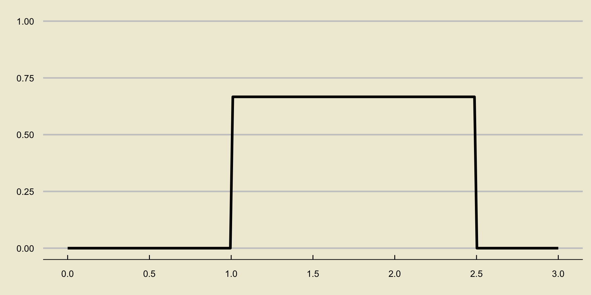
Oftentimes, we will be a bit lazy with our density curve and omit the open/closed circles. For example, we might sketch the density curve of the \(\mathrm{Unif}(1, \ 2.15)\) distribution as

Effect of Changing \(a\) and \(b\)

viewof a = Inputs.range(
  [-3, 3], 
  {value: 0, step: 0.1, label: "a="}
)

viewof b = Inputs.range(
  [-3, 3], 
  {value: 1, step: 0.1, label: "b="}
)

margin2 = ({top: 20, right: 30, bottom: 30, left: 40})

height2 = 400

x_values2 = d32.scaleLinear()
.domain(d32.extent(data2, d => d.x))
.range([margin2.left, width - margin2.right])

y_values2 = d32.scaleLinear()
.domain([Math.min(d32.min(data2, d => d.y),0), Math.max(1,d32.max(data2, d => d.y))]).nice()
.range([height2 - margin2.bottom, margin2.top])

line2 = d32.line()
.x(d => x_values2(d.x))
.y(d => y_values2(d.y))

xAxis2 = g => g
.attr("transform", `translate(0,${height2 - margin2.bottom})`)
.call(d32.axisBottom(x_values2)
      .ticks(width / 80)
      .tickSizeOuter(0))

yAxis2 = g => g
.attr("transform", `translate(${margin2.left},0)`)
.call(d32.axisLeft(y_values2)
      .tickValues(d32.scaleLinear().domain(y_values2.domain()).ticks()))

function unif_pdf (input_value, mu, sigsq) {
if(input_value < a){
  return 0
} else if(input_value > b){
  return 0
} else{
  return 1 / (b - a)
}
}

abs_x2=6

data2 = {
  let values = [];
  for (let x = -abs_x2; x < abs_x2; x=x+0.01) values.push({"x":x,"y":unif_pdf(x, µ, sigsquared)});
  return values;
}

d32 = require("https://d3js.org/d3.v5.min.js")

chart2 = {
  const svg = d32.select(DOM.svg(width, height2));
  
  svg.append("g")
  .call(xAxis2);
  
  svg.append("g")
  .call(yAxis2);
  
  svg.append("path")
  .datum(data2)
  .attr("fill", "none")
  .attr("stroke", "steelblue")
  .attr("stroke-width", 4)
  .attr("stroke-linejoin", "round")
  .attr("stroke-linecap", "round")
  .attr("d", line);
  
  return svg.node();
}

Credit to https://observablehq.com/@dswalter/normal-distribution for the base of the applet code

Uniform Probabilities

Recall, from our initial discussion on continuous random variables, that probabilities are found as areas underneath the density curve.
Due to the rectangular shape of the Uniform density curves, finding probabilities under the Uniform distribution ends up being relatively straightforward (so long as we remember how to find the area of a rectangle!)
Let’s work through an example together.

Worked-Out Example 1

If \(X \sim \mathrm{Unif}(-1, \ 1)\), compute \(\mathbb{P}(X \leq 0.57)\).

Solution

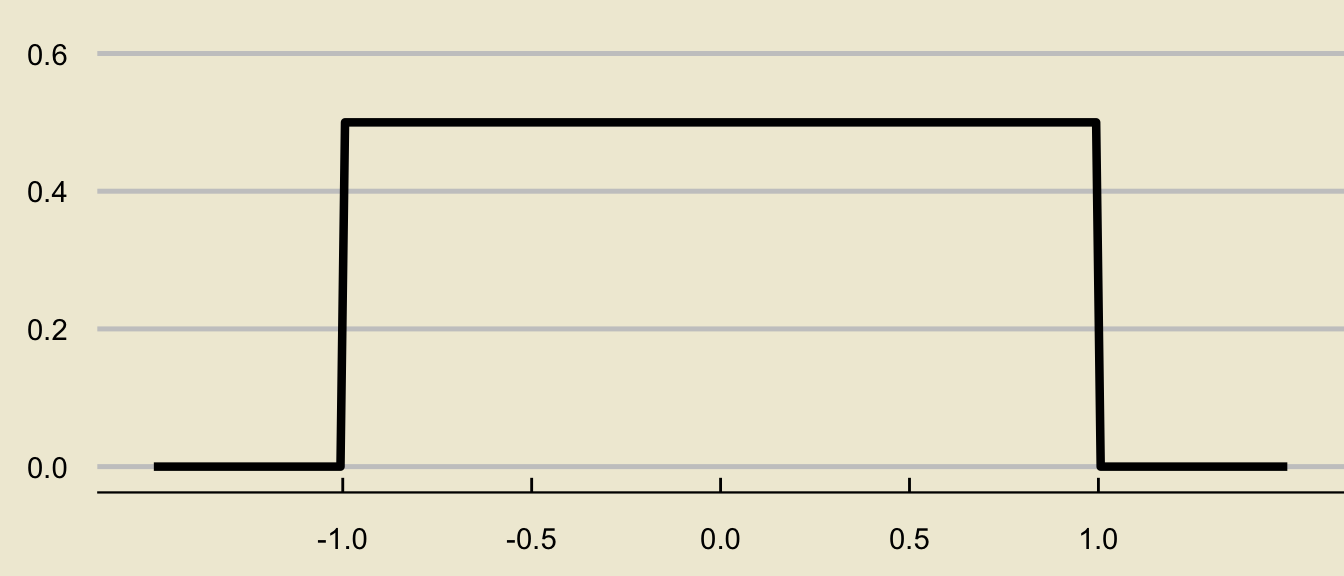
When working through probability problems involving continuous distributions, sketching a picture is always a good first step.
- Sometimes, we will explicitly make that the first step of a problem, meaning failure to sketch a relevant picture may result in less-than-full marks!
The density curve of the \(\mathrm{Unif}(-1, \ 1)\) distribution is given by

Solution

The desired probability is thus

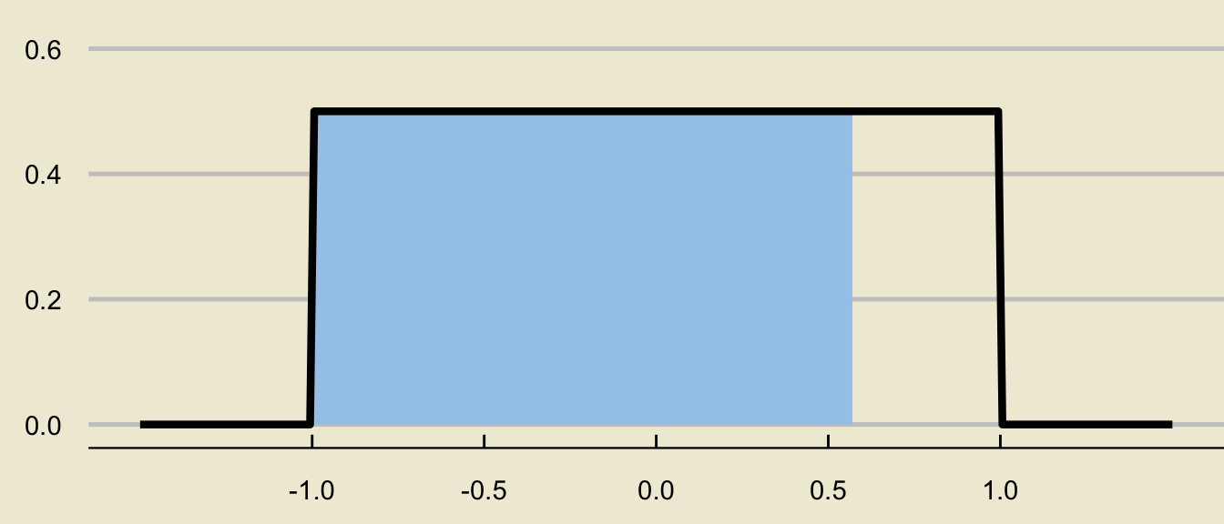
This is a rectangle with base \((0.57 - (-1)) = 1.57\) and height \(1 / (1 - (-1)) = 1/2\). Therefore, the area of this rectangle - and, also, the desired probability - is \[ (1.57) \times \frac{1}{2} = \boxed{0.785 = 78.5\%} \]

Another Example

Worked-Out Example 2

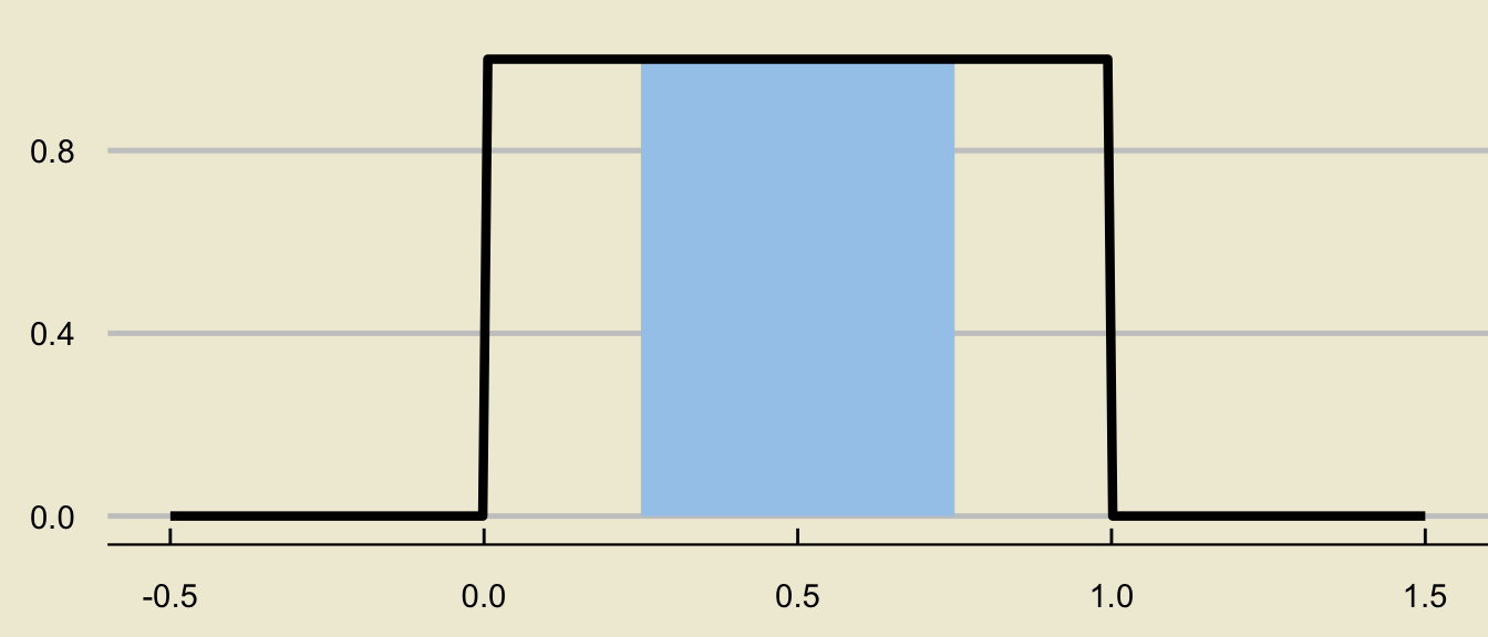
If \(X \sim \mathrm{Unif}(0, 1)\), compute \(\mathbb{P}(0.25 \leq X \leq 0.75)\).

We are going to solve this problem in two different ways.
Again, we always begin with a sketch of the desired probability as an area underneath the density curve:

This is a rectangle with base \((0.75 - 0.25) = 0.5\) and height \(1 / (1 - 0) = 1\), meaning its area is \[ (0.5) \cdot \left(1 \right) = \boxed{0.5 = 50\%} \]

Another way we can think about this area, however, is as a difference of two areas:

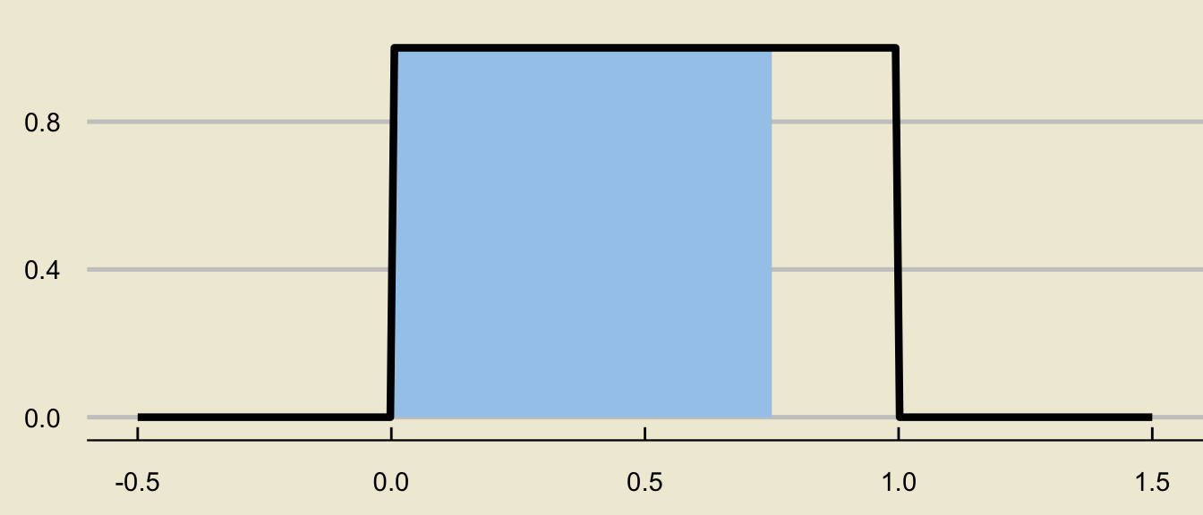
\[ \huge - \]

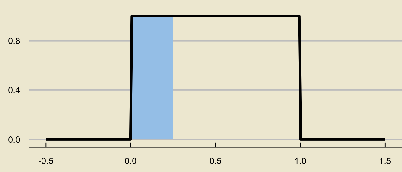
Tail Probabilities

This is not a coincidence!
For a more arbitrary distribution:

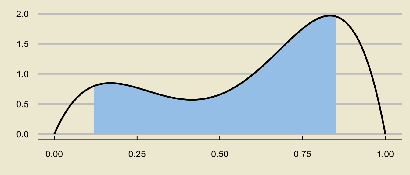
can be decomposed as

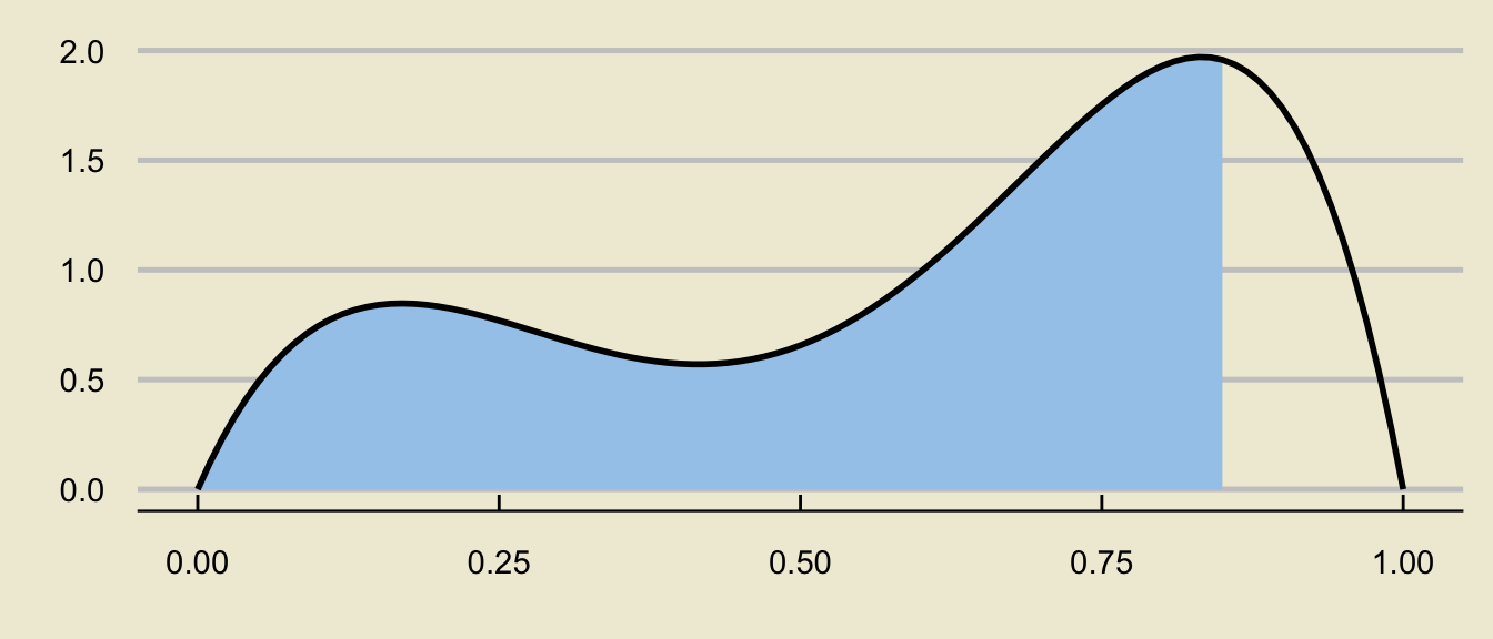
\[ \huge - \]

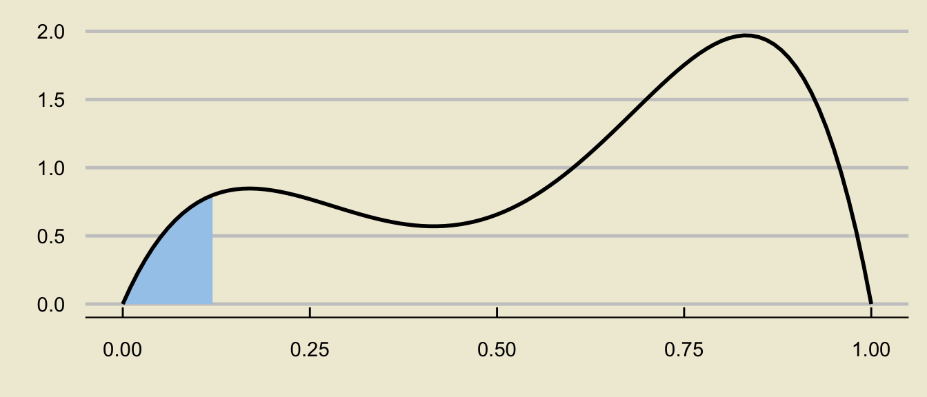
Tail Probabilities

In math, what we have found is:

Important

\[ \mathbb{P}(x_1 \leq X \leq x_2) = \mathbb{P}(X \leq x_2) - \mathbb{P}(X \leq x_1) \]

The quantity \(\mathbb{P}(X \leq x)\), where we view \(x\) as an arbitrary input (and hence the quantity \(\mathbb{P}(X \leq x)\) as a function of \(x\)) is called the cumulative distribution function (or c.d.f. for short) of \(X\).

Your Turn!

Exercise 2

The time (in minutes) spent waiting in line at Starbucks is found to vary uniformly between 5mins and 15mins.

Define the random variable of interest, and call it \(X\).
If a person is selected at random from the line at Starbucks, what is the probability that they spend between 3 and 7 minutes waiting in line?
Optional What is the c.d.f. of wait times? (I.e., find the probability that a randomly selected person spends less than \(x\) minutes waiting in line, for an arbitrary value \(x\). Yes, your final answer will depend on \(x\); that’s why the c.d.f. is a function!)

Probability of Attaining an Exact Value

If \(X \sim \mathrm{Unif}[0, 1]\), what is the probability that \(X\) equals, say \(0.5\)?
- The area this corresponds to is a rectangle of height \(1 / (1 - 0) = 1\), but with width \(0\).
- Therefore, the probability is zero.
This is not unique to the Uniform distribution!

Probability of Attaining an Exact Value

If \(X\) is a continuous random variable, \(\mathbb{P}(X = x) = 0\) for any value \(x\).

Mean and Variance of the Uniform Distribution

If \(X \sim \mathrm{Unif}[a, b]\), we have the following results:
- \(\displaystyle \mathbb{E}[X] = \frac{a + b}{2}\)
- \(\displaystyle \mathrm{Var}(X) = \frac{1}{12}(b - a)^2\)

Exercise 3

Consider again the setup of Exerise 2: the time (in minutes) spent waiting in line at Starbucks is found to vary uniformly on between 5mins and 15mins.

If we select a person at random, what is the expected amount of time (in minutes) they will spend waiting in line? What about the variance and standard deviation of the time (in minutes) they will spend waiting in line?

Normal Distribution

The normal distribution takes two parameters \(\mu\) and \(\sigma\). We use the notation \(X \sim \mathcal{N}(\mu, \ \sigma)\) to denote “\(X\) follows the normal distribution with parameters \(\mu\) and \(\sigma\).”
The normal distribution has distribution function given by \[ f(x) = \frac{1}{\sigma \cdot \sqrt{2 \pi}} \cdot \exp\left\{ - \frac{1}{2} \cdot \left( \frac{x - \mu}{\sigma} \right)^2 \right\} \]
Let’s determine how the parameters affect the shape of the density curve.

Changing \(\mu\) and \(\sigma\)

viewof µ = Inputs.range(
  [-3, 3], 
  {value: 0, step: 0.1, label: "µ:"}
)

viewof σ = Inputs.range(
  [0.2, 3.1], 
  {value: 1, step: 0.01, label: "σ:"}
)

sigsquared = σ**2

margin = ({top: 20, right: 30, bottom: 30, left: 40})

height = 400

x_values = d3.scaleLinear()
    .domain(d3.extent(data, d => d.x))
    .range([margin.left, width - margin.right])

y_values = d3.scaleLinear()
    .domain([Math.min(d3.min(data, d => d.y),0), Math.max(1,d3.max(data, d => d.y))]).nice()
    .range([height - margin.bottom, margin.top])
    
line = d3.line()
    .x(d => x_values(d.x))
    .y(d => y_values(d.y))

xAxis = g => g
  .attr("transform", `translate(0,${height - margin.bottom})`)
  .call(d3.axisBottom(x_values)
      .ticks(width / 80)
      .tickSizeOuter(0))

yAxis = g => g
  .attr("transform", `translate(${margin.left},0)`)
  .call(d3.axisLeft(y_values)
      .tickValues(d3.scaleLinear().domain(y_values.domain()).ticks()))
    
function normal_pdf (input_value, mu, sigsq) {
  let left_chunk = 1/(Math.sqrt(2*Math.PI*sigsq))
  let right_top = -((input_value-mu)**2)
  let right_bottom = 2*sigsq
  return left_chunk * Math.exp(right_top/right_bottom)
}

abs_x=6

data = {
  let values = [];
  for (let x = -abs_x; x < abs_x; x=x+0.01) values.push({"x":x,"y":normal_pdf(x, µ, sigsquared)});
  return values;
}

d3 = require("https://d3js.org/d3.v5.min.js")

chart = {
  const svg = d3.select(DOM.svg(width, height));

  svg.append("g")
      .call(xAxis);

  svg.append("g")
      .call(yAxis);
  
  svg.append("path")
      .datum(data)
      .attr("fill", "none")
      .attr("stroke", "steelblue")
      .attr("stroke-width", 4)
      .attr("stroke-linejoin", "round")
      .attr("stroke-linecap", "round")
      .attr("d", line);
  
  return svg.node();
}

Credit to https://observablehq.com/@dswalter/normal-distribution for the majority of the applet code

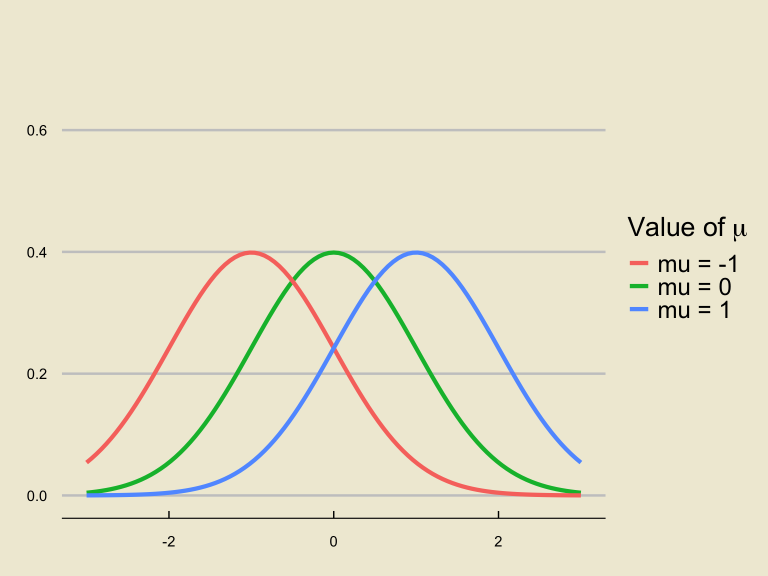
Changing \(\mu\)

Holding \(\sigma = 1\) fixed and varying \(\mu\), we find:

Changing \(\sigma\)

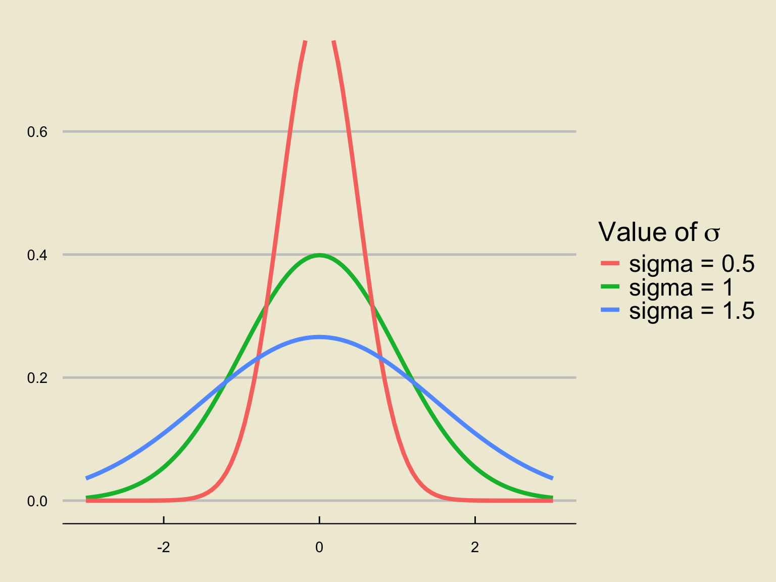
Holding \(\mu = 0\) fixed and varying \(\sigma\), we find:

Standard Normal Distribution

Definition

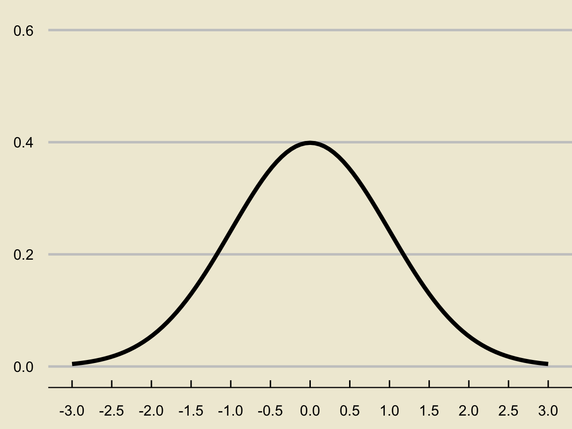
The standard normal distribution is the normal distribution with \(\mu = 0\) and \(\sigma = 1\); i.e. \(\mathcal{N}(0, 1)\).

Normal Probabilities

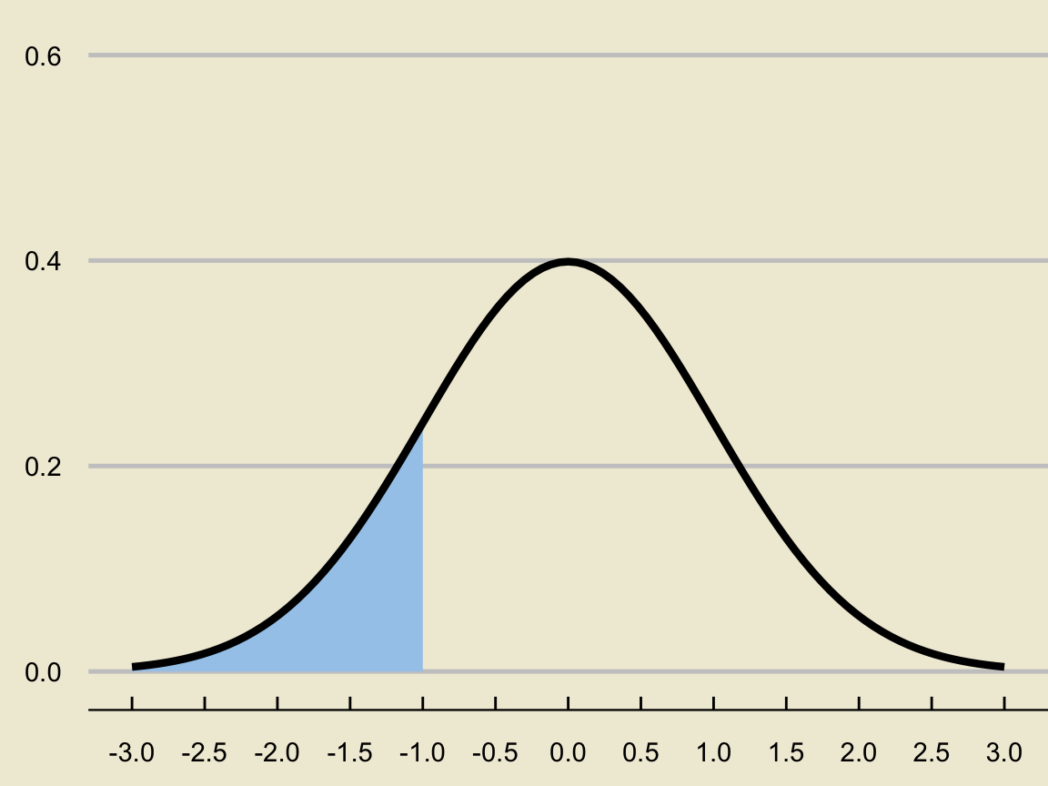
Recall that for continuous variables, probabilities are found as areas underneath the density curve. For example, if \(X \sim \mathcal{N}(0, 1)\), then \(\mathbb{P}(X \leq -1)\) is found by computing the area below:

Normal Probabilities

Now, unlike with the Uniform density curve, we don’t have a simple closed-form formula for areas under the Normal curve.
For instance, how would you get a numerical value for the area shaded on the previous slide?
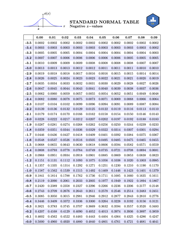
The answer is by way of what is known as a normal table, or z-table.
To illustrate how to read a normal table, let’s work through an example:

Worked-Out Example 3

If \(Z \sim \mathcal{N}(0, 1)\), compute \(\mathbb{P}(Z \leq 0.83)\).

Normal Table

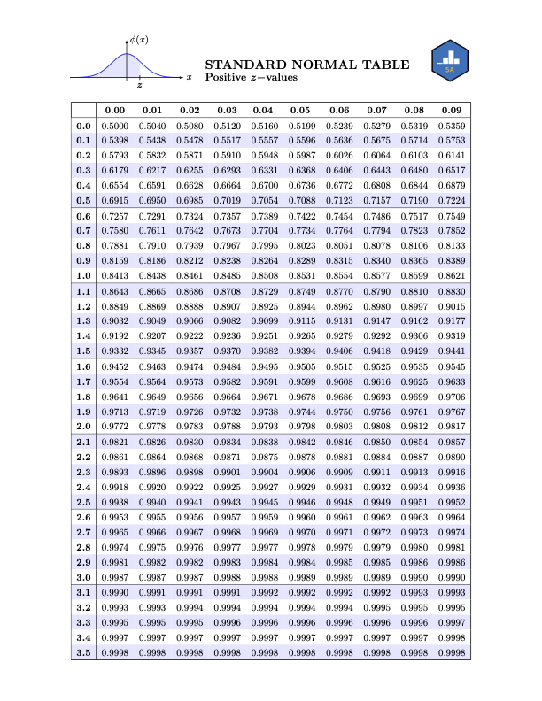
Reading the Normal Table

To find \(\mathbb{P}(Z \leq 0.83)\), we break up \(0.83\) as \[ 0.83 = 0.8 + 0.03 \]
This tells us to find the desired probability in the intersection of the \(0.8\) row and the \(0.03\) column:

Another Example

Worked-Out Example 4

If \(Z \sim \mathcal{N}(0, 1)\), find

\(\mathbb{P}(Z \leq -1.01)\)
\(\mathbb{P}(Z \leq -2.25)\)
\(\mathbb{P}(-2.25 \leq Z \leq -1.01)\)
\(\mathbb{P}(X \geq -0.7)\)

Standardization

Now, all of our considerations above were in the case of the standard normal distribution. How do we find areas under nonstandard normal density curves?
The answer: we use a process called standardization.

Standardization

If \(X \sim \mathcal{N}(\mu, \ \sigma)\), then \[ \left( \frac{X - \mu}{\sigma} \right) \sim \mathcal{N}(0, 1) \] That is, if we take a normally distributed random variable, subtract off its mean, and divide by its standard deviation, we obtain a random variable whose distribution is the standard normal distribution.

The act of taking a random variable, subtracting its mean, and dividing by its standard deviation is known as standardization.

In the context of the normal distribution, the standardized value of a number \(x\) (i.e. \((x - \mu)/\sigma\)) is called a z-score.
- Note that the \(z-\)score of a value \(x\) measures how many standard deviations \(x\) was from the mean.

Normal Probabilities; General Case

Thus, if \(X \sim \mathcal{N}(\mu, \ \sigma)\), here are the steps we use to compute \(\mathbb{P}(X \leq x)\):
1. Compute the \(z-\)score \(z = \frac{x - \mu}{\sigma}\), rounded to two decimal places.
2. Look up the corresponding entry in a standard normal table.

Worked-Out Example 5

If \(X \sim \mathcal{N}(5, \ 1.21)\), compute \(\mathbb{P}(X \leq 6)\).

The \(z-\)score of \(6\) is \[ z = \frac{6- 5}{1.21} \approx 0.83 \]
Looking up the probability corresponding to \(0.83\) on a standard normal table (which we did in Worked-Out Example 3), we see that the desired probability is \(\boxed{0.7967 = 79.67\%}\)

Your Turn!

Exercise 4

It is found that the scores on a particular exam are normally distributed with a mean of 83 and a standard deviation of 5.

Define the random variable of interest, and call it \(X\).
If a student is selected at random, what is the probability that they scored 81 or lower?
If a student is selected at random, what is the probability that they scored 75 or higher?

Mean and Variance of the Normal Distribution

If \(X \sim \mathcal{N}(\mu, \ \sigma)\), we have the following results:
- \(\displaystyle \mathbb{E}[X] = \mu\)
- \(\displaystyle \mathrm{Var}(X) = \sigma^2\)
So, the two parameters we use to describe the normal distribution are the mean and the variance.
We’ll talk more about parameters in the next lecture.