PSTAT 5A: Lecture 12

Further Inference on Proportions

Ethan P. Marzban

2023-07-13

Last Time

Last time we began discussing inference on a proportion.
We had a population with proportion \(p\), drew representative samples from this population, and used the sample proportion \(\widehat{P}\) (i.e. the proportion observed in the sample) as a proxy for \(p\).
Our main result was the Central Limit Theorem for Proportions which states \[ \widehat{P} \sim \mathcal{N}\left( p, \ \sqrt{ \frac{p(1 - p)}{n} } \right) \] assuming the success-failure conditions are met:
1. \(np \geq 10\)
2. \(n(1 - p) \geq 10\)

Substitution Approximation

Can anyone point out a potential difficulty with verifying the success-failure conditions?
That’s right; they involve the parameter \(p\), which is in many cases unknown!
- Remember - in the beginning of last lecture, I mentioned that the whole point of performing statistical inference is to try and make claims about a population parameter that is unknowable, or too difficult to determine exactly.
To remedy this, we often use the so-called substitution approximation to the success-failure conditions:
1. \(n \widehat{p} \geq 10\)
2. \(n(1 - \widehat{p}) \geq 10\)
Sometimes, we substitute \(\widehat{p}\) into the formula for the standard deviation of \(\widehat{P}\), as the next example illustrates.

Worked-Out Example

Worked-Out Example 1

A veterinarian wishes to determine the true proportion of cats that suffer from FIV (Feline Immunodeficiency Virus). To that end, she takes a representative sample of 500 cats and finds that 3.2% of cats in this sample have FIV. What is the probability that the proportion of cats that are FIV-positive in her sample of 500 cats lies within 1 percent of the true proportion of FIV-positive cats?

Solution

Let \(p\) denote the true proportion of FIV-positive cats. Let \(\widehat{P}\) denote the proportion of FIV-positive cats in a representative sample of size 500.
- Do we know the value of \(p\)?
- No we do not.
What we do have is \(\widehat{p} = 0.032\).
- Therefore, we use the substitution approximation to the success-failure conditions:
- \(n \widehat{p} = (500)(0.032) = 16 \geq 10 \ \checkmark\)
- \(n (1 - \widehat{p}) = (500)(1 - 0.032) = 484 \geq 10 \ \checkmark\)
Since both conditions are met, the CLT tells us \[ \widehat{P} \sim \mathcal{N}\left(p, \ \sqrt{\frac{p(1 - p)}{500}} \right)\]

Solution

We seek \(\mathbb{P}(p - 0.01 \leq \widehat{P} \leq p + 0.01)\).
Our first step is to write this as \[ \mathbb{P}(\widehat{P} \leq p + 0.01) - \mathbb{P}(\widehat{P} \leq p - 0.01 ) \]
Next, we find the associated \(z-\)scores: \[\begin{align*} z_1 & = \frac{(p + 0.01) - p}{\sqrt{\frac{p(1 - p)}{500}}} = \frac{0.01}{\sqrt{\frac{p(1 - p)}{500}}} \\ z_2 & = \frac{(p - 0.01) - p}{\sqrt{\frac{p(1 - p)}{500}}} = - \frac{0.01}{\sqrt{\frac{p(1 - p)}{500}}} \end{align*}\]

Solution

Now, we can apply the substitution approximation to plug in \(\widehat{p}\) in place of \(p\) in the denominator of our \(z-\)scores to compute \[\begin{align*} z_{1, \ \text{sub}} & = \frac{0.01}{\sqrt{\frac{(0.032)(1 - (0.032))}{500}}} = \frac{0.01}{0.00787} = 1.27 \\ z_{2, \ \text{sub}} & = - \frac{0.01}{\sqrt{\frac{(0.032)(1 - (0.032))}{500}}} = - \frac{0.01}{0.00787} = -1.27 \end{align*}\]
Finally, consulting our standard normal table, we find the answer to be \[ 0.8980 - 0.1020 = \boxed{0.796 = 79.6\%} \]

A Note

I’d like to stress that the substitution approximation is just that- an approximation.
It is not, for instance, true that \(\mathbb{E}[\widehat{P}] = \widehat{p}\); the center of the distribution of \(\widehat{P}\) will always (provided the success-failure conditions are met) be \(p\), the true value of the proportion.

Leadup

Let’s quickly take stock of what we’ve learned.
If we have a population with some unknown population parameter \(p\), we can repeatedly take representative samples, compute the sample proportion in each sample, and construct the sampling distribution of \(\widehat{P}\).
Assuming the success-failure conditions are met, this sampling distribution will be centered at \(p\), the true proportion value, and hence a decent estimator for \(p\) would be \(\mathbb{E}[\widehat{P}]\).

Leadup

However, the key assumption in this procedure is our ability to take multiple samples from the population.
In many practical situations, this is not feasible.
So, here is a new question to consider: given just a single sample from the population, what can we say about \(p\)?
Well, we’ve already seen that it’s risky to simply take \(\widehat{p}\) (i.e. the value of \(\widehat{P}\) that was observed in the sample we took) to be an estimate of \(p\), due to the randomness associated with \(\widehat{P}\).
Instead of looking for point estimates of \(p\), what happens if we instead provide intervals we believe may contain \(p\)?

Leadup

Let’s make things a bit more concrete. Since I like cats, let’s go back to our veterinarian example:

A veterinarian wishes to determine the true proportion of cats that suffer from FIV (Feline Immunodeficiency Virus). To that end, she takes a representative sample of 100 cats and finds that 3.2% of cats in this sample have FIV.

Again, it’s risky to say that “the true proportion of FIV-positive cats is 3.2%” based solely on this sample.
Instead, we are going to start proposing intervals of values that we believe contain \(p\).
Now, clearly the strengths of our beliefs will depend on the interval we provide.
For example, I am 100% confident that the true proportion of FIV-positive cats is somewhere in the interval \((-\infty, \infty)\).
But, suppose we instead consider the interval \((0.030, \ 0.034)\); now we can’t really say that we’re 100% certain this interval covers the true value of \(p\).

Confidence Intervals

This is the basic idea of what are known as confidence intervals.
I particularly like the analogy our textbook (OpenIntro Statistics) uses:

[…] Using only a point estimate is like fishing in a murky lake with a spear. We can throw a spear where we saw a fish, but we will probably miss. On the other hand, if we toss a net in that area, we have a good chance of catching the fish. (page 181)

For the purposes of this class, we will construct confidence intervals for an arbitrary parameter \(\theta\) (e.g. a population proportion \(p\), a population mean \(\mu\), etc.) of the form \(\widehat{\theta} \pm \mathrm{m.e.}\) where \(\widehat{\theta}\) represents some point estimate of \(\theta\) and \(\mathrm{m.e.}\) represents a margin of error.
So, for the veterinarian example, our confidence interval will be of the form \(\widehat{p} \pm \mathrm{m.e.}\).

Confidence Intervals

Before constructing a confidence interval, however, we need to specify our confidence level. In other words, we need first have an idea of how confident we want to be that our interval contains the true parameter value.
For example, a 95% confidence interval is an interval \(\widehat{\theta} \pm \mathrm{m.e.}\) that we are 95% confident covers the true value of \(\theta\).
Here’s a question: based on everything we’ve talked about thus far, do you think higher confidence levels correspond to wider or narrower intervals?
- That’s right: the higher our confidence level, the wider our interval will be.
- As an extreme example, consider again the slightly absurd confidence interval \((-\infty, \ \infty)\); this is a 100% confidence interval because we are 100% confident that it covers the true value of the parameter!
So, therein lies the tradeoff: the more confidence we want, the wider we need to make our intervals and the less informative they become in pinning down the true value of the parameter.

Confidence Intervals for Proportions

Alright, let’s return to our considerations on population proportions.
Again, our confidence interval will take the general form \(\widehat{p} \pm \mathrm{m.e.}\).
It makes sense that the margin of error should include some information about the variability of \(\widehat{P}\). As such, we take our confidence intervals to be of the form \[ \widehat{p} \pm z^{\ast} \cdot \sqrt{ \frac{p(1 - p)}{n} } \] where \(z^{\ast}\) is a constant that depends on our confidence level.
- \(z^{\ast}\) is sometimes called the confidence coefficient, though that name is not fully standard.

Confidence Intervals for Proportions

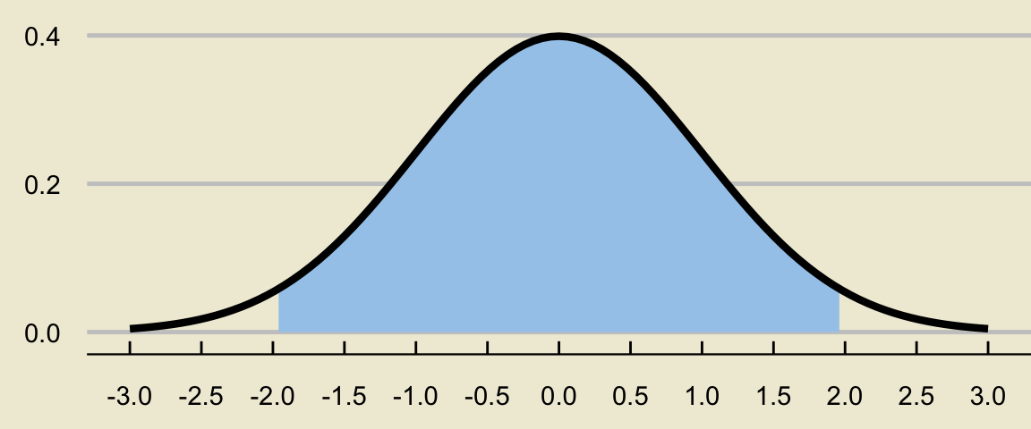
To see exactly how this dependency manifests itself, let’s make things a bit more concrete and consider a 95% confidence level. It turns out that this implies \[ \mathbb{P}(-z^{\ast} \leq Z \leq z^{\ast}) = 0.95 \] where \(Z \sim \mathcal{N}(0, \ 1)\).
- I’ll try to post some supplementary material for those of you curious as to why this is- for now, I ask you to just take this fact at face value.
As always, we draw a picture.

Confidence Intervals for Proportions

The region we will sketch is the area under the standard normal curve between \(-z^{\ast}\) and \(z^{\ast}\):

Now, here’s the slightly peculiar thing- in this case, we know that the area itself must be 0.95. What we don’t know is exactly where those endpoints are.

Confidence Intervals for Proportions

Some of you may have an inkling that a normal table may be helpful…. and it will be!
To make clear how a normal table will help, let’s convert our picture to be in terms of tail areas:

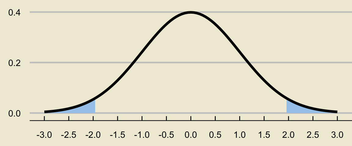
What must be the area of the shaded bit above?
- That’s right: 5% (since the area in the middle is, by construction, 95%).

Confidence Intervals for Proportions

Because the standard normal density curve is symmetric, the area of any one of the two tails must be (5% / 2) = 2.5%:

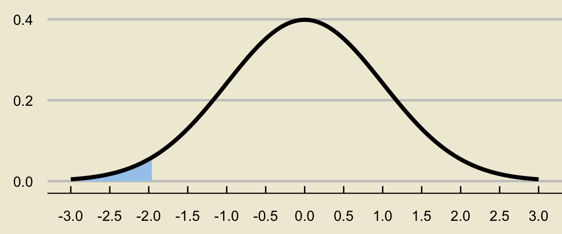
So, what we have shown, is that \(z^{\ast}\) must satisfy the condition \[ \mathbb{P}(Z \leq -z^{\ast}) = 0.025 \]

Confidence Intervals for Proportions

Again, \(z^{\ast}\) must satisfy \[ \mathbb{P}(Z \leq -z^{\ast}) = 0.025 \]
From a normal table, we see that \[ \mathbb{P}(Z \leq -1.96) = 0.025 \]
Therefore, we must have \[ \mathbb{P}(Z \leq -z^{\ast}) = \mathbb{P}(Z \leq -1.96) \] that is, \(-z^{\ast} = -1.96\) or \(\boxed{z^{\ast} = 1.96}\).

Confidence Intervals for Proportions

So, in conclusion, a 95% confidence interval for a population proportion will take the form \[ \widehat{p} \pm 1.96 \cdot \sqrt{ \frac{p(1 - p)}{n} } \]

Exercise 2

Use a similar set of reasoning to show that a 90% confidence interval for a population proportion \(p\) takes the form \[ \widehat{p} \pm 1.645 \cdot \sqrt{\frac{p(1 - p)}{n}} \]

Quick Aside: Percentiles of the Standard Normal Distribution

As a quick aside: notice that what we’ve done is actually found various percentiles of the standard normal distribution!
Percentiles of a distribution are defined much in the same way we defined the percentiles of a list of numbers: the p^th percentile of a random variable \(X\) is the value \(\pi_p\) such that \(\mathbb{P}(X \leq \pi_p) = p\).
To find the p^th percentile of the standard normal table, here are the steps we use:
1. Find \(p\) in the body of the table
2. Whatever \(z-\)score that corresponds to the value of \(p\) in the table will be the p^th percentile

Exercise 3

Find the 4.55^th, 83.4^th, and 96.41^th percentiles of the standard normal distribution.

Symmetry of the Normal Distribution

Let’s also quickly discuss one more property of the standard normal distribution: its density curve is symmetric about the \(y-\)axis.
This actually leads to an interesting (and very useful) result about percentiles of the standard normal distribution:

Result

The \(p\)^th percentile of the standard normal distribution is equal to negative one times the \((1 - p)\)^th percentile of the standard normal distribution.

Symmetry of the Normal Distribution

To see why this is, we sketch a picture. Suppose \(\pi_{p}\) is the \(p\)^th percentile for the standard normal distribution. Then, the area below must be equal to \(p\):

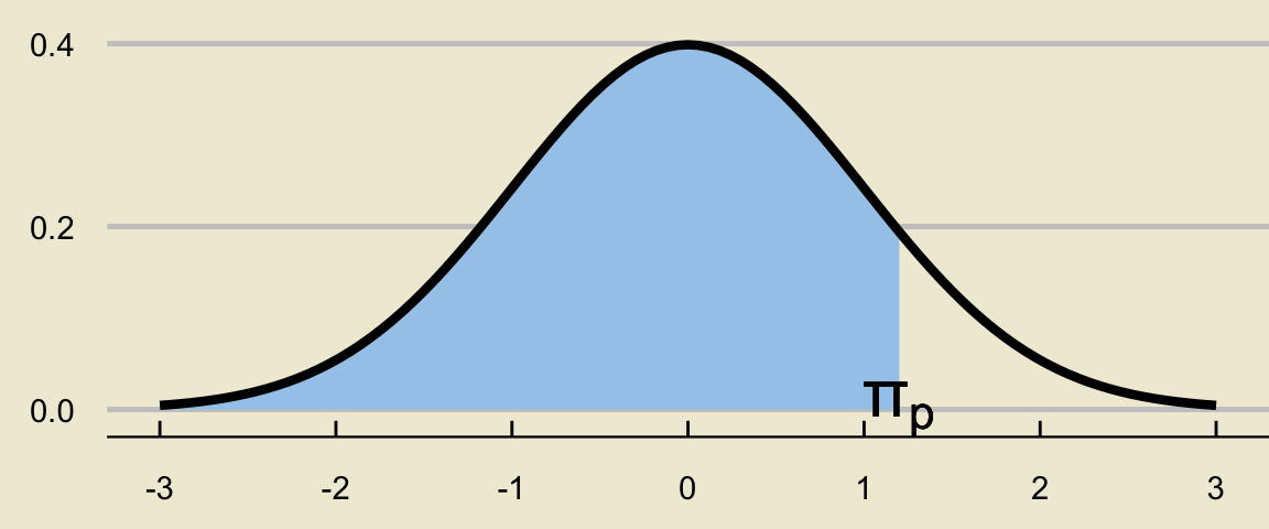
Symmetry of the Normal Distribution

By the complement rule, the red area below must therefore be \(1 - p\):

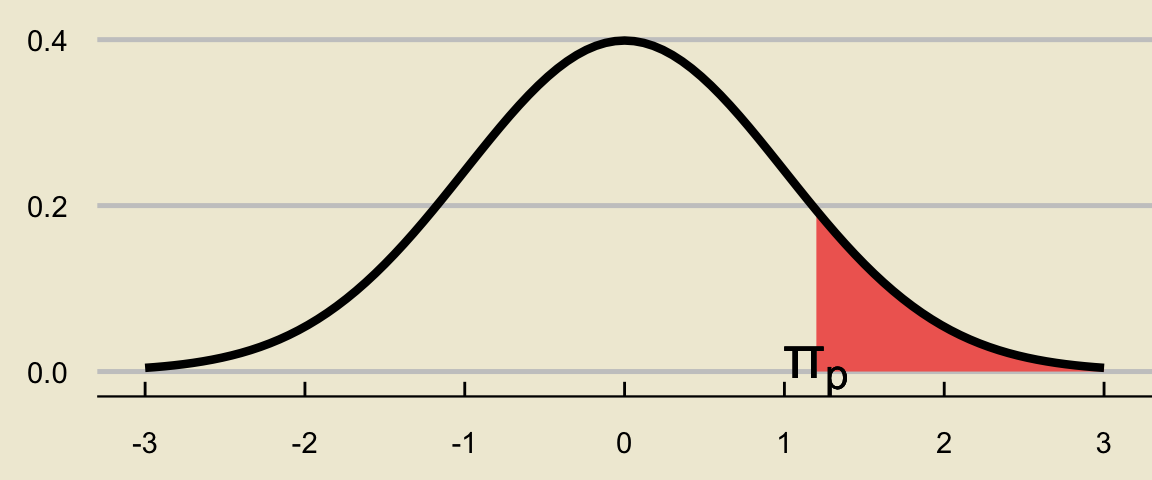
Symmetry of the Normal Distribution

Finally, it is precisely the symmetry of the standard normal density curve that guarantees the red area below will also be \(1 - p\):

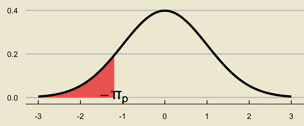
Therefore, if the area to the left of \(\pi_p\) is \(p\) (which was our initial assumption), the area to the left of \(-\pi_p\) is \((1 - p)\).
- In other words, the \(p\)^th percentile (\(\pi_p\)) is negative one times the \((1 - p)\)^th percentile (\(-\pi_p\)).

Confidence Intervals for Proportions

Here are some common confidence levels, and their corresponding values of \(z^{\ast}\).

Confidence Level	Value of \(\boldsymbol{z^{\ast}}\)
90%	1.645
95%	1.96
99%	2.575

Recall that these \(z^{\ast}\)’s are simply corresponding percentiles (scaled by \(-1\)) of the standard normal distribution.
To find \(z^{\ast}\) corresponding to an arbitrary \(100 \times (1 - \alpha)\) interval we either:
- find the \((\alpha / 2) \times 100\)^th percentile of the standard normal distribution and multiply by \((-1)\)
- find the \([1 - (\alpha / 2)] \times 100\)^th percentile of the standard normal distribution.

Confidence Intervals for Proportions

For example, suppose we want to construct a 99% confidence interval.
This is equivalent to constructing a \((1 - 0.01) \times 100\%\) confidence interval, meaning to find the confidence coefficient we can:
- find the \((0.01 / 2) \times 100 = 0.5\)^th percentile of the standard normal distribution and scale by \(-1\), which yields a value of around \(2.575\)
- find the \([1 - (0.01 / 2)] \times 100 = 99.5\)^th percentile of the standard normal distribution, which (again) yields a value of around \(2.575\)

Confidence Intervals for Proportions

In practice: since the value of \(p\) is unknown, we typically replace \(p\) with \(\widehat{p}\) to obtain an approximate confidence interval: \[ \widehat{p} \pm z^{\ast} \cdot \sqrt{ \frac{\widehat{p}(1 - \widehat{p})}{n}} \]

Worked-Out Example

Worked-Out Example 2

A veterinarian wishes to determine the true proportion of cats that suffer from FIV (Feline Immunodeficiency Virus). To that end, she takes a representative sample of 500 cats and finds that 3.2% of cats in this sample have FIV. Construct a 95% confidence interval for the true poportion of FIV-positive cats.

We simply plug into our formula from above: \[ (0.032) \pm 1.96 \cdot \sqrt{ \frac{(0.032) \cdot (1 - 0.032)}{500}} = \boxed{0.032 \pm 0.0155}\] or, written out more explicitly, \[ \boxed{ [0.0165 \ , \ 0.0475] } \]

Interpreting Confidence Intervals

Okay, now that we have an example of a confidence interval under our belt, let’s talk about the correct interpretation of confidence intervals.
The following are all correct interpretations of our confidence interval:
- We are 95% confident that the true proportion of FIV-positive cats is between 0.0165 and 0.0475.
- We are 95% confident that the interval \([0.0165 \ , \ 0.0475]\) covers the true proportion of FIV-positive cats.
Here is a technically incorrect way of interpreting the confidence interval: there is a 95% probability that the true proportion of FIV-positive cats lies between 0.0165 and 0.0475.

Interpreting Confidence Intervals

Why is this typically rejected as an interpretation of a confidence interval?
Because this phrasing makes it sound as though the true proportion of FIV-positive cats is a random variable!
- The true proportion of FIV positive cats is a fixed, deterministic value \(p\).
- What is random are the endpoints of our confidence interval!
- This is why we phrase our interpretation in terms of “coverage”; it is to highlight the fact that the endpoints of our interval are where our uncertainty (i.e. randomness) comes into play.
I grant that the above is a very subtle point. However, Statisticians are quite particular about wording when it comes to interpreting confidence intervals. As such, we will be particular in this class as well!

Your Turn!

Exercise 3

As a film critic, you are interested in determining the true proportion of people that have watched The Mandalorian. You take a representative sample of 100 people, and note that 47% of these people have watched The Mandalorian.

Construct a 95% confidence interval for the proportion of people that have watched The Mandalorian, and interpret your interval in the context of the problem.
When constructing an 85% confidence interval for the proportion of people that have watched The Mandalorian, would you expect this interval to be wider or shorter than the interval you found in part (a)?
Now, actually construct an 85% confidence interval for the proportion of people that have watched The Mandalorian and see if this agrees with your answer to part (b).

Your Turn!

Exercise 4

As a political scientist, Morgan would like to know the true proportion of people in a city that support Candidate A in an upcoming election. To that effect, they take a representative sample of 120 people and determine that 51% of these sampled individuals support Candidate A.

Construct an 87% confidence interval for the true proportion of people that support Candidate A.