PSTAT 5A: Lecture 21

Regression, Part II

Ethan P. Marzban

2023-07-31

Last Time

• Last time, we began our foray into statistical modeling.

• Given data \(\{(x_i, \ y_i)\}_{i=1}^{n}\) on a response variable y and an explanatory variable x, we model the relationship between y and x as \[ \texttt{y} = f(\texttt{x}) + \texttt{noise} \] for some signal function \(f()\).

• When the response variable is numerical, we call the model a regression model; when the variable is categorical, we call the model a classification model.

• Ulimately, we wish to fit a signal function \(\widehat{f}()\) to our data.

Simple Linear Regression

• Simple Linear Regression refers to a situation in which we have:

  • a numerical response variable y
  • a single explanatory variable x
  • a linear signal function; i.e. \(f(x) = \beta_0 + \beta_1 \cdot x\)

• That is, the model in a simple linear regression setting is \[ \texttt{y} = \beta_0 + \beta_1 \cdot x + \texttt{noise} \]

  • Fitting a signal function \(\widehat{f}()\) to the data is therefore equivalent to finding suitable estimators \(\widehat{\beta}_0\) and \(\widehat{\beta}_1\) of \(\beta_0\) and \(\beta_1\) respectively.

A Note/Connection

• I’d like to stress- writing \(f(x) = \beta_0 + \beta_1 \cdot x\) is exactly the same as our familiar \(mx + b\) form for a line!

  • The reason we use \(\beta_0\) and \(\beta_1\) in place of \(b\) and \(m\), respectively, is to allow for an extension of the same notation practices to a multivariate setting.

  • That is, if we have \(k\) explanatory variables x₁ through x_k, it is easier to write a linear model as \[ \texttt{y} = \beta_0 + \beta_1 \cdot x_1 + \cdots + \beta_k \cdot x_k + \texttt{noise} \] instead of having to find new letters for the coefficients of x₁ through x_k.

OLS Estimators and the OLS Regression Line

• Back to the model fitting problem: we seek to find “good” estimators \(\widehat{\beta}_0\) and \(\widehat{\beta}_1\) for \(\beta_0\) and \(\beta_1\) respectively.

• One quantification of “good” is “minimizing the residual sum of squares”:

\[ \mathrm{RSS} = \sum_{i=1}^{n} e_i^2 \]

OLS Estimators and the OLS Regression Line

• The estimators that minimize the RSS are \[\begin{align*} \widehat{\beta}_1 & = \frac{\sum\limits_{i=1}^{n} (x_i - \overline{x})(y_i - \overline{y})}{\sum\limits_{i=1}^{n} (x_i - \overline{x})^2} \\ \widehat{\beta}_0 & = \overline{y} - \widehat{\beta}_1 \overline{x} \end{align*}\] which are called the ordinary least squares (or just OLS) estimators of \(\beta_0\) and \(\beta_1\).

• We write the OLS regression line as \[ \widehat{y} = \widehat{\beta}_0 + \widehat{\beta}_1 \cdot x \] which is just the line that “best” fits the data (where, again, “best” is quantified by minimizing the RSS).

Correlation?

• By the way: remember that we also talked about Pearson’s correlation coefficient last lecture.

• It is defined as \[ r = \frac{1}{n - 1} \sum_{i=1}^{n} \left( \frac{x_i - \overline{x}}{s_X} \right) \left( \frac{y_i - \overline{y}}{s_Y} \right) \] and gives a way of quantifying the strength of the linear association between two lists of numbers \(\{x_i\}_{i=1}^{n}\) and \(\{y_i\}_{i=1}^{n}\).

• I mentioned last time that \(r\) does NOT give the slope of the line that best fits the data- that role is given to \(\widehat{\beta}_1\)!

• However, there is in fact a connection between \(\widehat{\beta}_1\) and \(r\): it turns out (after a bit of math), we can equivalently compute \(\widehat{\beta}_1\) as \[ \widehat{\beta} = \frac{s_Y}{s_X} \cdot r \]

Fitted Values

• We also introduced the notion of fitted values:

• This is why we write the OLS regression line as \[ \widehat{y} = \widehat{\beta}_0 + \widehat{\beta}_1 \cdot x \] the fitted values are simply the points along the OLS regression line!

Prediction

• In this way, we can perhaps see how the OLS regression line can be used to perform prediction.

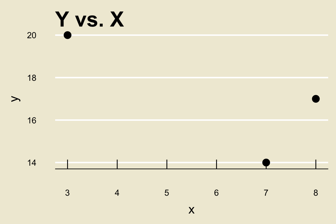
• To see how this works, let’s return to a toy example from last lecture: \[\begin{align*} \boldsymbol{x} & = \{3, \ 7, \ 8\} \\ \boldsymbol{y} & = \{20, \ 14, \ 17\} \end{align*}\]

Prediction

• Notice that we do not have an x-observation of 5. As such, we don’t know what the y-value corresponding to an x-value of 5 is.

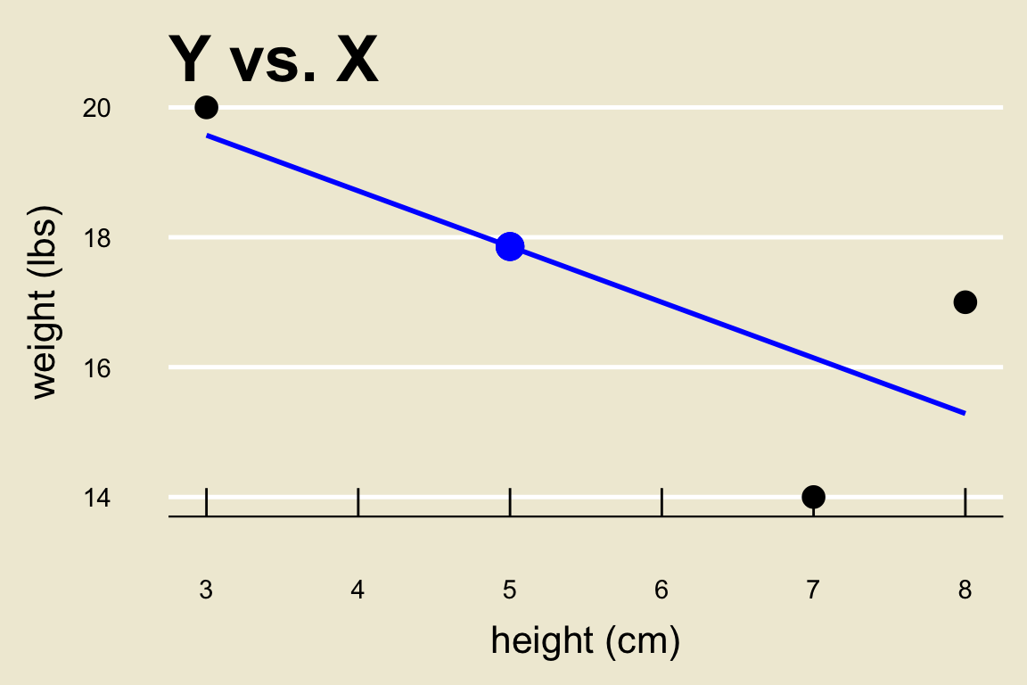
• However, we do have a decent guess as to what the y-value corresponding to an x-value of 5 is- the corresponding fitted value!

Prediction

• In other words, our best guess at (i.e. our best prediction of) the \(y-\)value corresponding to an \(x-\)value of \(5\) is the point \(\widehat{y}^{(5)}\) obtained by plugging \(x = 5\) into the OLS regression line:

\[ \widehat{y}^{(5)} = \frac{1}{7} (155 - 6 \cdot 5) \approx 17.857 \]

Leadup

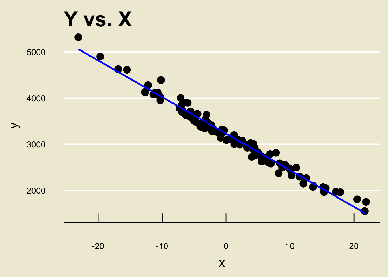
• Let’s look at another toy dataset:

Leadup

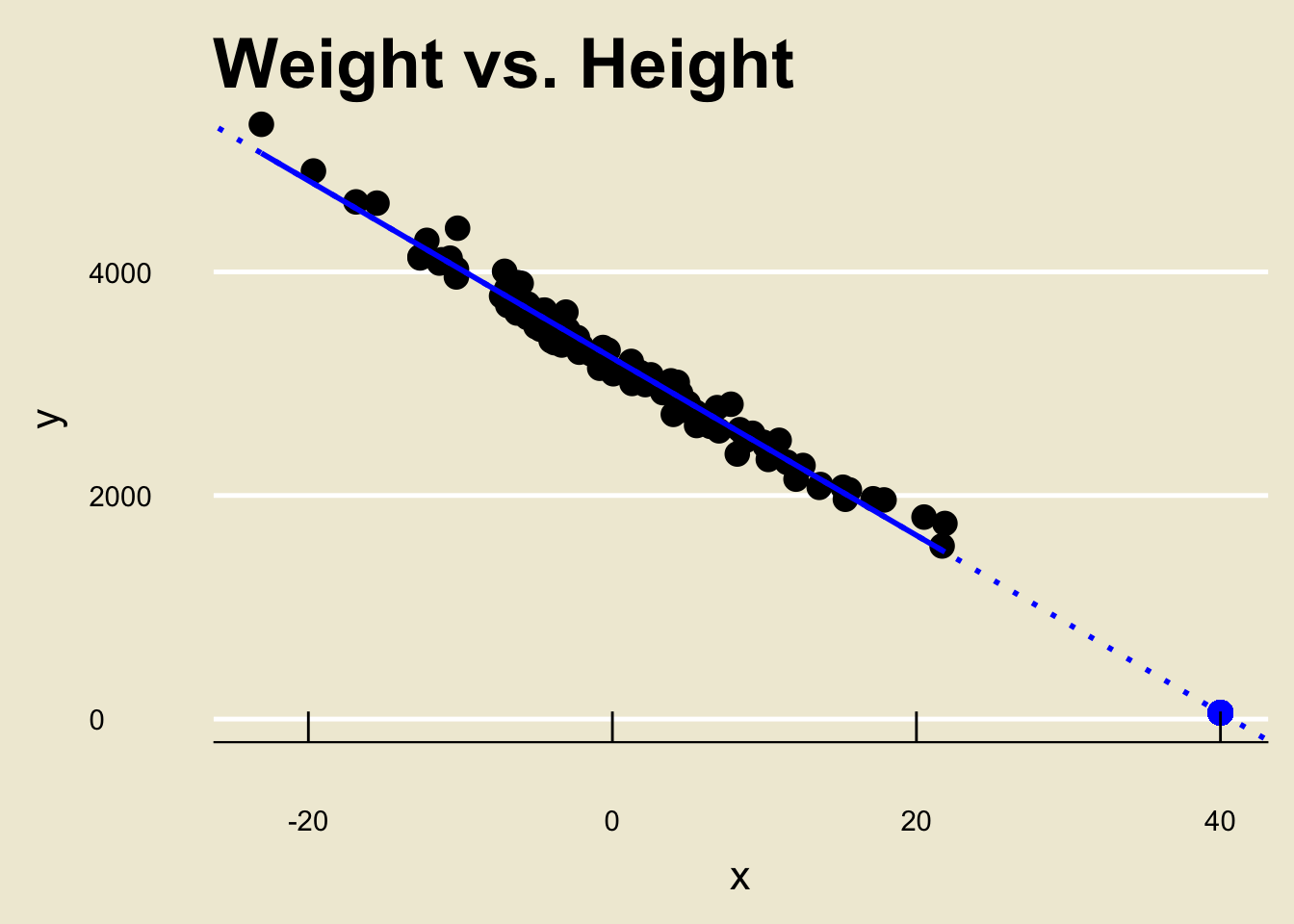
• Say we want to predict the corresponding y value of an x value of, 40.

• Following our steps from before, we would just find the fitted value corresponding to x = 40:

Leadup

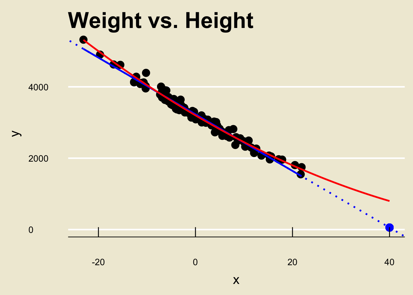
• Here’s the kicker: the true fit was actually NOT linear!

Extrapolation, and the Dangers Thereof

• Specifically, the true signal function was quadratic. (When you zoom in close enough, parabolas look linear!)

• This is why it is a bad idea to try to extrapolate too far.

  • Extrapolation is the name we give to trying to apply a model estimate to values that are very far outside the realm of the original data.

  • How far is “very far”? Statisticians disagree on this front. For the purposes of this class, just use your best judgment.

Your Turn!

Exercise 1

An airline is interested in determining the relationship between flight duration (in minutes) and the net amount of soda consumed (in oz.). Letting x denote flight duration (the explanatory variable) and y denote amount of soda consumed (the response variable), a sample yielded the following results: \[ \begin{array}{cc} \displaystyle \sum_{i=1}^{102} x_i = 20,\!190.55; & \displaystyle \sum_{i=1}^{102} (x_i - \overline{x})^2 = 101,\!865 \\ \displaystyle \sum_{i=1}^{102} y_i = 166,\!907.8 & \displaystyle \sum_{i=1}^{102} (y_i - \overline{y})^2 = 120,\!794.2 \\ \displaystyle \sum_{i=1}^{100} (x_i - \overline{x})(y_i - \overline{y}) = 80,\!184.62 \\ \end{array} \]

1. Find the equation of the OLS Regression line.
2. If a particular flight has a duration of 130 minutes, how many ounces of soda would we expect to be consumed on the flight? (Suppose the \(x-\)observations ranged from around \(114\) to around \(271\))

Back to \(\widehat{\beta}_1\)

• Recall that, by virtue of being the slope of the OLS regression line, \(\widehat{\beta}_1\) has the following interpretation:

A one-unit change in x corresponds to a predicted \(\widehat{\beta}_1\)-unit change in y.

• Notice the word “predicted” there- remember that \(\widehat{\beta}_1\) is an estimator, not the true slope!

  • That is to say: different datasets generated from the same model may produce different values of \(\widehat{\beta}_1\).

• That’s right: \(\widehat{\beta}_1\) can be thought of as a random variable.

Back to \(\widehat{\beta}_1\)

• We know that \(\widehat{\beta}_1\) seeks to estimate \(\beta_1\).

• It seems plausible, then, that we might be able to perform inference on \(\beta_1\) (the true slope) using \(\widehat{\beta}_1\) (the OLS estimator).

• Indeed, we can!

• Let’s start off by considering confidence intervals for the true slope \(\beta_1\).

Confidence Intervals for \(\beta_1\)

• Recall that (at least in the confines of this course), given a parameter \(\theta\) and an estimator \(\widehat{\theta}\) of \(\theta\), we construct a confidence interval for \(\theta\) as \[ \widehat{\theta} \pm c \cdot \mathrm{SD}(\widehat{\theta}) \] where \(c\) is a constant that depends on both the sampling distribution of \(\widehat{\theta}\) along with the confidence level.

• This means we can construct a confidence interval for \(\beta_1\) using \[ \widehat{\beta}_1 \pm c \cdot \mathrm{SD}(\widehat{\beta}_1) \] where \(\widehat{\beta}_1\) is the OLS estimator of \(\beta_1\).

Confidence Intervals for \(\beta_1\)

• It turns out that finding \(\mathrm{SD}(\widehat{\beta}_1)\) is fairly involved. As such, I won’t expect you to compute it- you will be provided with its value for a given problem (see the practice problems for an example of what I mean).

• We also need access to the sampling distribution of \(\widehat{\beta}_1\).

• Assuming both the x-observations and y-observations are roughly normal, then \[ \frac{\widehat{\beta}_1 - \beta_1}{\mathrm{SD}(\widehat{\beta_1})} \sim t_{n - 2} \]

• This means our critical value should be the appropriately-selected quantiles of the t_n-2 distribution.

Worked-Out Example

Worked-Out Example 1

Consider the same setup as Exercise 1. Suppose it is known that \[ \mathrm{Var}(\widehat{\beta}_1) \approx 0.006135 \] Construct a 95% confidence interval for \(\beta_1\), the true amount of change in y (amount of soda consumed) associated with a one-unit change in x (flight duration)

Solutions

• We previously saw that \(\widehat{\beta}_1 \approx 0.7871656\).

• We know to use the \(t_{100}\) distribution; since we are using a 95% confidence level, we take \(1.98\) as our confidence coefficient (make sure you know where this came from!)

• Hence, our confidence interval is \[(0.7871656) \pm 1.98 \cdot \sqrt{0.006135} = \boxed{[0.6321 \ , \ 0.9423]}\]

• The interpretation of this interval is similar to the interpretation of our confidence intervals thus far:

We are 95% confident that the interval \([0.6321 \ , \ 0.9423]\) covers the true value of \(\beta_1\).

Example

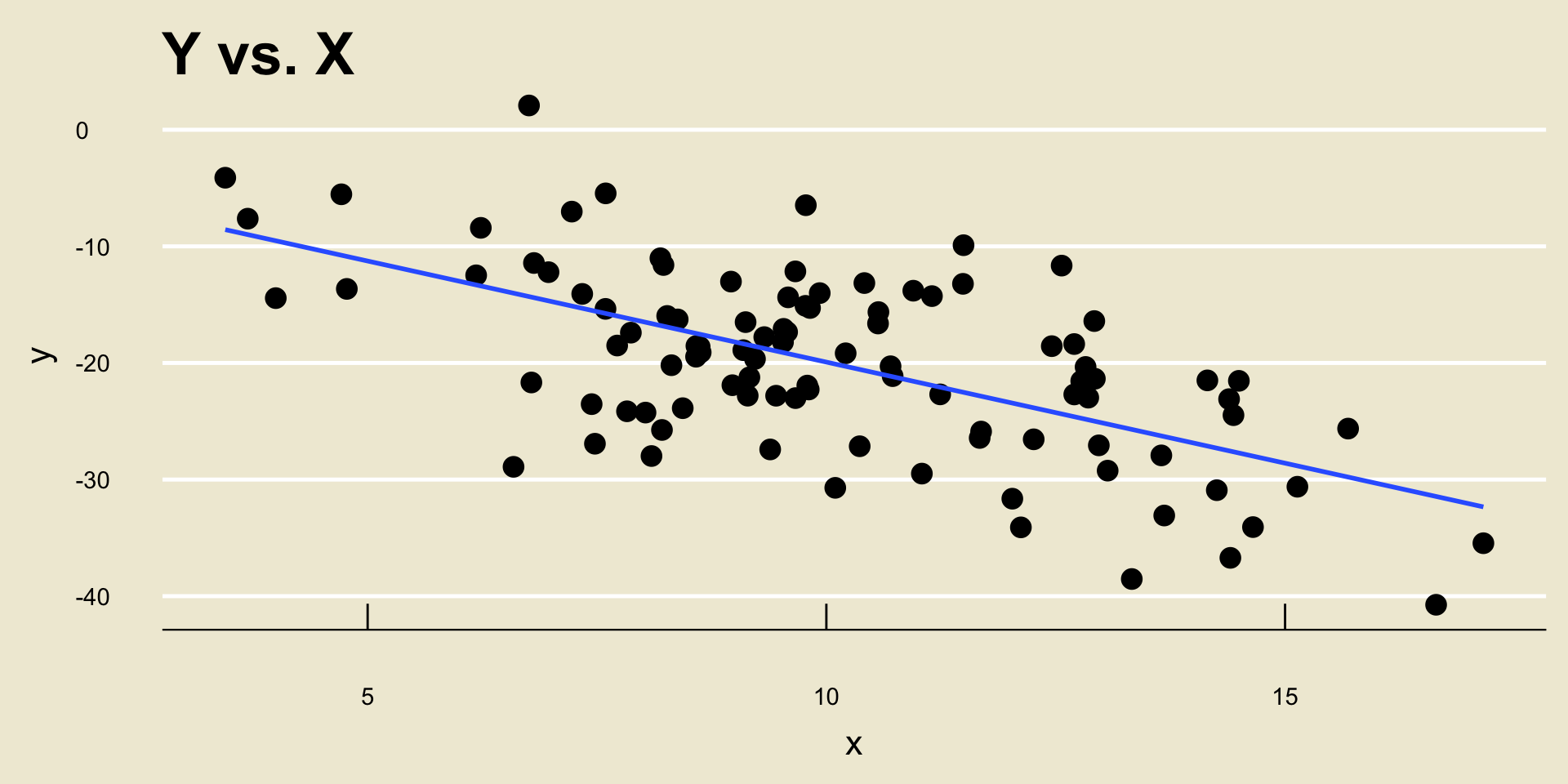
• \(\widehat{\beta_0} =\) -2.5884231; \(\widehat{\beta_1} =\) -1.733778

Example

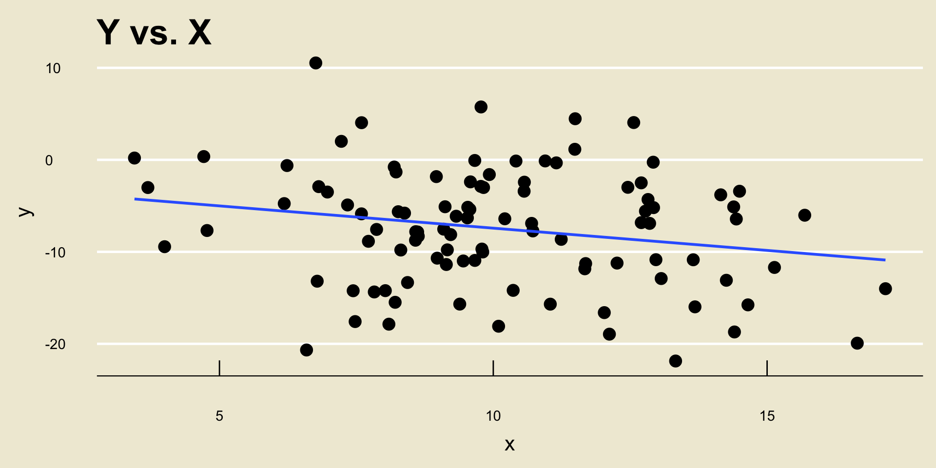
• \(\widehat{\beta_0} =\) -2.5884231; \(\widehat{\beta_1} =\) -0.483778

Example

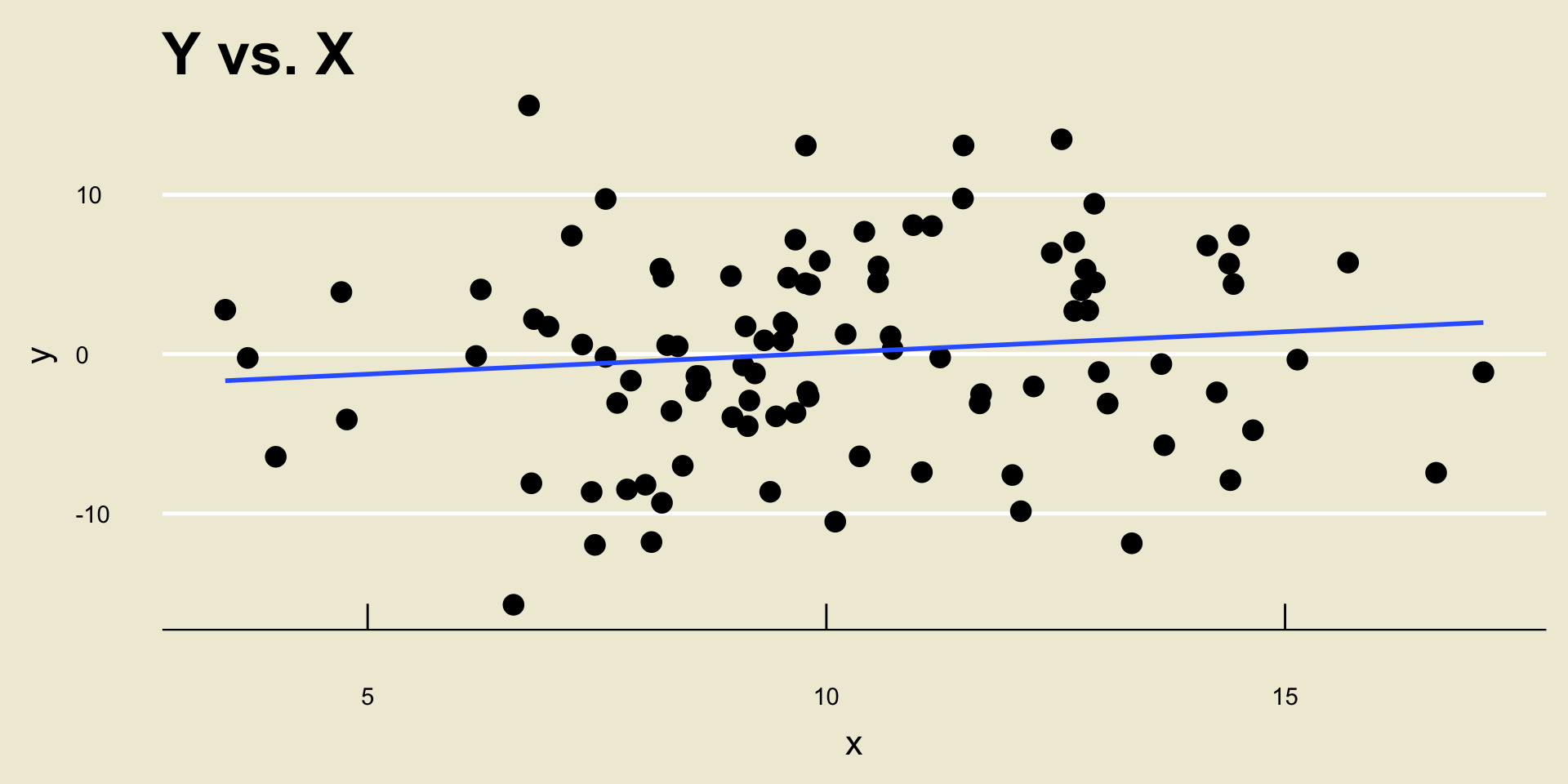
• \(\widehat{\beta_0} =\) -2.5884231; \(\widehat{\beta_1} =\) 0.266222

• Do we really believe the slope, though?

Leadup

• Without the OLS regression line, the scatterplot on the previous page would likely be one we classify as exhibiting “no relationship” between x and y.

• However, the OLS regression line has picked up a positive slope.

• What’s going on?

• In other words, does our data (i.e. the data that gave rise to the value of \(\widehat{\beta}_1\) computed) support our claim that there is no relationship?

Hypothesis Testing on \(\beta_1\)

• What do you know- we’ve entered the realm of hypothesis testing!

• Specifically, we are trying to use our data to test the hypotheses \[ \left[ \begin{array}{rl} H_0: & \beta_1 = 0 \\ H_A: & \beta_1 \neq 0 \end{array} \right. \]

  • Why is our null \(\beta_1 = 0\)?
  • Well, our null is that there is no relationship.
  • Recall that \(\beta_1\) is the slope of the linear relationship assumed to exist between y and x.
  • Hence, saying “no relationship” is equivalent to saying “a change in x corresponds to no change in y”; i.e. that \(\beta_1 = 0\).

Hypothesis Testing on \(\beta_1\)

• We already have a pretty good candidate for a test statistic: \[ \mathrm{TS} = \frac{\widehat{\beta}_1}{\mathrm{SD}(\widehat{\beta}_1)} \] since, under the null, this follows a \(t_{n - 2}\) distribution: \[ \mathrm{TS} = \frac{\widehat{\beta}_1}{\mathrm{SD}(\widehat{\beta}_1)} \stackrel{H_0}{\sim} t_{n - 2} \]

Hypothesis Testing on \(\beta_1\)

• Our test then takes the form \[ \texttt{decision}(\mathrm{TS}) = \begin{cases} \texttt{reject } H_0 & \text{if } |\mathrm{TS}| > c \\ \texttt{fail to reject } H_0 & \text{otherwise}\\ \end{cases} \] where \(c\) is the appropriately-selected quantile of the t_n-2 distribution.

• Equivalently, we compute p-values using the t_n-2 distribution.

Hypothesis Testing on \(\beta_1\)

• Indeed, many computer softwares (and statistical papers!) report a table resembling the following after running a regression:

	Estimate	Std. Error	t-value	Pr(>|t|)
Intercept	-2.588	2.327	-1.112	0.269
Slope	-1.734	0.222	-7.811	6.41e-12

• The first column is the raw estimated value (i.e. \(\widehat{\beta_0}\) and \(\widehat{\beta_1}\), respectively)

• The second column is the standard error (i.e. standard deviation) of the estimator

• The third column is the test statistic (i.e. the first column divided by the second)

• The fourth column is the p-value in a two-sided test, testing whether or not the given parameter is actually zero or not.

Let’s Play Around with Regression in Python

Task

• Here’s a task for you: write a function called regtab() that takes in two inputs, x and y, and returns a regression table resulting from regressing y on x.

  • You can use the scipy.stats.linregress() function

Some Exercises

Exercise 2 (modified from StatClass)

Consider the following regression equation, obtained from a sample of size \(50\): \[ \widehat{y} = 3.8 - 0.277 x \] and the standard deviation of \(\widehat{\beta}_1\) is 0.39.

Using a 5% level of significance, perform a test of the hypotheses \[ \left[ \begin{array}{rl} H_0: & \beta_1 = 0 \\ H_A: & \beta_1 \neq 0 \end{array} \right.\]

Some Exercises

Exercise 3 (modified from StatClass)

Ten towns were the subject of a study to determine whether or not an increased number of stores selling liquor in their downtown areas is linked with a higher number of DUI arrests downtown during one month. The data and summary information is provided below.

x	0	5	6	5	11	9	10	3	7	4
y	40	50	55	64	73	75	88	25	20	10

\[ \begin{array}{lll} \overline{x} = 6 & \displaystyle \sum_{i=1}^{10} (x_i - \overline{x})^2 = 102 \\ \overline{y} = 50 & \displaystyle \sum_{i=1}^{10} (y_i - \overline{y})^2 = 6,\!024 & \displaystyle \sum_{i=1}^{10} (x_i - \overline{x})(y_i - \overline{y}) = 513 \end{array} \]

1. What is the explanatory variable?
2. What is the response variable?
3. Find the equation of the OLS regression line.
4. If the standard deviation of \(\widehat{\beta}_1\) is \(0.37\), construct a 95% confidence interval for \(\beta_1\).
5. Is the slope significant? (Use the standard deviation from part (d) if necessary.)